Mapping input noise to escape noise in integrate-and-fire neurons: a level-crossing approach [original]

Biological Cybernetics (2021) 115:539–562

https://doi.org/10.1007/s00422-021-00899-1

ORIGINAL ARTICLE

Mapping input noise to escape noise in integrate-and-fire neurons: a

level-crossing approach

Tilo Schwalger1,2

Received: 17 July 2021 / Accepted: 27 September 2021 / Published online: 19 October 2021

Abstract

Noise in spiking neurons is commonly modeled by a noisy input current or by generating output spikes stochastically with a

voltage-dependent hazard rate (“escape noise”). While input noise lends itself to modeling biophysical noise processes, the

phenomenological escape noise is mathematically more tractable. Using the level-crossing theory for differentiable Gaussian

processes, we derive an approximate mapping between colored input noise and escape noise in leaky integrate-and-fire

neurons. This mapping requires the first-passage-time (FPT) density of an overdamped Brownian particle driven by colored

noise with respect to an arbitrarily moving boundary. Starting from the Wiener–Rice series for the FPT density, we apply the

second-order decoupling approximation of Stratonovich to the case of moving boundaries and derive a simplified hazard-rate

representation that is local in time and numerically efficient. This simplification requires the calculation of the non-stationary

auto-correlation function of the level-crossing process: For exponentially correlated input noise (Ornstein–Uhlenbeck process),

we obtain an exact formula for the zero-lag auto-correlation as a function of noise parameters, mean membrane potential and

its speed, as well as an exponential approximation of the full auto-correlation function. The theory well predicts the FPT and

interspike interval densities as well as the population activities obtained from simulations with colored input noise and time-

dependent stimulus or boundary. The agreement with simulations is strongly enhanced across the sub- and suprathreshold

firing regime compared to a first-order decoupling approximation that neglects correlations between level crossings. The

second-order approximation also improves upon a previously proposed theory in the subthreshold regime. Depending on a

simplicity-accuracy trade-off, all considered approximations represent useful mappings from colored input noise to escape

noise, enabling progress in the theory of neuronal population dynamics.

Keywords Integrate-and-fire neuron ·Interspike interval density ·First-passage-time density ·Colored noise ·Escape noise ·

Hazard rate ·Threshold-crossing statistics ·Neuronal population dynamics

1 Introduction

Neurons in the brain must operate under highly non-

stationary conditions. In fact, most behaviorally relevant

sensory stimuli as well as internal signals are rarely con-

stant in time but may change rapidly. In the presence of

noise, such dynamic stimuli can be reliably encoded in the

time-dependent population activity of a large population of

Communicated by Moritz Helias.

BTilo Schwalger

[email protected]

1Institute of Mathematics, Technical University Berlin, 10623

Berlin, Germany

2Bernstein Center for Computational Neuroscience Berlin,

10115 Berlin, Germany

spiking neurons (Gerstner et al. 2014). The time-dependent

population activity also provides a concise coarse-grained

description of the collective dynamics of interacting spik-

ing neurons. Therefore, theories that predict the population

activity in response to a time-dependent signal have been

of fundamental interest in theoretical neuroscience (Knight

1972; Gerstner 2000; Augustin et al. 2017; Schwalger et al.

2017).

The population activity of noisy spiking neurons can be

mathematically described by population density equations

(Nykamp and Tranchina 2000; Chizhov 2017). The form

of the population density equation depends on the noise

model. Two popular ways to model neuronal noise consist

of modeling noise either in the input or in the output of the

neuron (Gerstner et al. 2014). In the first model class (input

noise), noise enters the dynamical equations of the membrane

123

540 Biological Cybernetics (2021) 115:539–562

potential, currents or conductances leading to stochastic dif-

ferential equations. If the noise is Gaussian white noise, the

subthreshold dynamics becomes a diffusion process and the

input noise is also called diffusive noise (Gerstner 2000).

The corresponding population density equation is a Fokker–

Planck equation and the population activity can be obtained

as the probability flux across the threshold (Abbott and

van Vreeswijk 1993; Brunel and Hakim 1999; Fourcaud

and Brunel 2002; Nykamp and Tranchina 2000; Richard-

son 2008; Augustin et al. 2017). Models based on diffusive

noise naturally appear as the result of modeling biophysical

processes such as synaptic shot-noise or ion channel noise.

In particular, a frequently considered source of noise is back-

ground synaptic input modeled as external Poisson processes

(Brunel 2000; Potjans and Diesmann 2014). The fluctuating

part of this external shot noise leads, via a diffusion approxi-

mation (Gerstner et al. 2014), to Gaussian white noise driving

the synaptic input current or conductance. Besides its bio-

physical interpretability, input noise has the advantage that it

permits modeling both temporal (Fourcaud and Brunel 2002;

Schwalger et al. 2015) and spatial (Lindner et al. 2005) corre-

lations of synaptic inputs and enables mean-field theories for

recurrent networks of sparsely connected integrate-and-fire

neurons (Brunel and Hakim 1999; Brunel 2000).

In the second model class (called output noise or escape

noise (Gerstner 2000)), the dynamical equations for the state

variables are deterministic, while spikes (“output”) are gen-

erated stochastically through a hazard rate or conditional

intensity (Gerstner 2000; Paninski 2004; Truccolo et al.

2005; Pillow et al. 2008; Pillow and Latham 2008; Naud

and Gerstner 2012;Breaetal.2013; Galves and Löcherbach

2016; Gerhard et al. 2017; Raad et al. 2020). This hazard

rate depends on the state variables via a link function. For

example, it may be given as ˆ

λ(t)=Ψ(u(t), ˆ

t(t)), where

u(t)is the membrane potential and ˆ

t(t)is the last spike

time of the neuron at time t. If the neuron model is a

non-homogeneous renewal or quasi-renewal (Naud and Ger-

stner 2012) process, the corresponding population density

equation is a renewal integral equation or, equivalently, a

refractory density equation (Gerstner et al. 2014; Gerstner

2000; Naud and Gerstner 2012; Chizhov and Graham 2007,

2008; Dumont et al. 2016; Schwalger and Chizhov 2019).

Although output noise is of phenomenological nature without

a quantitative link to biophysical mechanisms, it has several

advantages (Schwalger and Chizhov 2019) owing to its sim-

pler mathematical tractability: First, the refractory density

or integral equation admits an extension to finite numbers

of neurons (Schwalger et al. 2017; Schwalger and Chizhov

2019; Schmutz et al. 2020,2021). This extension allows to

account for finite-size fluctuations of the population activ-

ity at the mesoscopic scale. Second, models with output

noise provide analytical expressions for the likelihood func-

tion, and thus, model parameters can be efficiently fitted

to experimental data of single neuron recordings (Panin-

ski 2004; Truccolo et al. 2005; Pillow et al. 2008; Gerhard

et al. 2017;Mensietal.2012; Pozzorini et al. 2015; Teeter

et al. 2018). And third, the state space for models with

output noise remains approximately one-dimensional even

for multi-dimensional conductance-based neuron models

(Chizhov and Graham 2007). The one-dimensional descrip-

tion permits highly efficient numerical solutions, in contrast

to Fokker–Planck equations (Apfaltrer et al. 2006), which

become intractable and computationally inefficient for sev-

eral state variables.

In view of the wide use of biologically interpretable input

noise and the mathematical advantages of output noise, an

intriguing question is whether input noise can be approxi-

mately mapped to output noise, so as to take full advantage

of both noise models. Mathematically, such a map requires

the specification of the hazard rate ˆ

λ(t)in terms of a link

function Ψ, which depends on some dynamical variables

and defines the escape-noise model. Unfortunately, a stan-

dard method to derive such a link function does not exist.

To see this, let us consider the example of non-homogeneous

renewal processes as a popular class of neuron models. In

these models, the probability density P(t|ˆ

t)to fire the next

spike at time tgiven a spike at time ˆ

t,ˆ

t<t, does not depend

on the state of the model before time ˆ

t, i.e., the memory

of renewal neurons only reaches back to its last spike. An

important example of non-homogeneous renewal models in

neuroscience are one-dimensional integrate-and-fire neurons

driven by white input noise (Gerstner et al. 2014). For this

model class one can formally construct the hazard rate via

the formula λ(t|ˆ

t)=P(t|ˆ

t)/1−t

tP(s|ˆ

t)ds(Gerstner

et al. 2014). However, there are two obstacles: first, in order

to apply this formula, the “interspike interval (ISI) density”

P(t|ˆ

t)would be needed in analytical form for arbitrary, time-

dependent input currents {I(t)}t∈(ˆ

t,t)that occurred since the

last spike. However, the calculation of the ISI density for

time-dependent inputs is equivalent to a first-passage-time

(FPT) problem with time-dependent parameters or boundary.

The solution of this FPT problem requires the solution of the

Fokker–Planck equation with moving absorbing boundary,

which is known to be a hard theoretical problem (Bulsara

et al. 1996; Schindler et al. 2004; Lindner 2004b). Second,

even if one succeeds to derive an approximate formula for

the hazard rate λ(t|ˆ

t), it is still challenging to represent the

hazard rate in the form of a link function Ψu(t), {z(t)},ˆ

t

that depends on some voltage-like variable u(t),thelast

spike time ˆ

tand possibly further dynamical variables {z(t)}

locally in time (as opposed to a “non-local” functional of

{u(t), z(t)}t∈(ˆ

t,t)).

Several theoretical studies have suggested approximate

local hazard rates for leaky integrate-and fire (LIF) models

driven by white (Plesser and Gerstner 2000; Herrmann and

Gerstner 2001; Chizhov and Graham 2007) or exponentially

123

Biological Cybernetics (2021) 115:539–562 541

correlated (Chizhov and Graham 2008) Gaussian noise, or

quasi-static (frozen) noise (Goedeke and Diesmann 2008).

In this paper, we explore an alternative approach to the haz-

ard rate and the first-passage-time density based on the theory

of level crossings (Verechtchaguina et al. 2006). In Sect. 2,

we introduce the LIF model with time-dependent driving

and constant threshold and map this process an equivalent

model with constant input and moving barrier. In Sect. 3,

we consider the level crossing statistics with respect to this

moving barrier and use the Wiener–Rice series and approx-

imations thereof to provide formal expressions for the FPT

density. These expressions form the starting point for deriv-

ing approximate hazard rates that are local in time. This

derivation reveals some unexpected results concerning the

correlations of level-crossings of Gaussian processes at small

time lags (Sect. 3.4). Then, we turn to the LIF model and the

problem of mapping input noise to escape noise (Sect. 4)

and apply this map to predict the time-dependent population

activity of LIF neurons with colored input noise (Sect. 5).

Each of the Sects. 3,4and 5closes with a comparison of the

level-crossing theory with simulations and a previous the-

ory by Chizhov and Graham (2008). Detailed derivations are

provided in Appendix.

2 Leaky integrate-and-fire models and the

associated first-passage-time problem

As a spiking neuron model with input noise, we consider a

leaky integrate-and-fire model driven by synaptically filtered

(“colored”) noise (Schwalger and Schimansky-Geier 2008;

Gerstner et al. 2014; Schuecker et al. 2015). In this model,

spikes are emitted whenever the membrane potential V(t)

reaches a threshold VT. The subthreshold dynamics for V<

VTcan be written as

τm˙

V=−V+μ(t)+η(t), (1a)

τs˙η=−η+2τsσηξ(t), (1b)

where τmis the membrane time constant and μ(t)=Vrest +

RI(t)is the mean neuronal drive consisting of a constant

resting potential Vrest and a time-dependent input current

I(t)(Rdenotes the membrane resistance). Furthermore, η(t)

is a colored noise modeled as a one-dimensional Ornstein–

Uhlenbeck process with correlation time τsand variance σ2

η,

and ξ(t)is a zero-mean Gaussian white noise with auto-

correlation function ξ(t)ξ(t)=δ(t−t). The colored

noise captures the effect of various intrinsic and extrinsic

noise sources, such as fluctuations of synaptic background

activity in vivo (shot noise due to random spike arrival from

background neurons). After threshold crossing and spike

emission, V(t)is reset to a reset potential VR,VR<VT, and

the subthreshold dynamics Eq. (1) resumes after an absolute

refractory period of length tref following the reset.

We are seeking a corresponding spiking neuron model

with escape-noise (Gerstner 2000) given by a hazard rate

(conditional intensity) of the form Ψu(t), ˙u(t), {zi(t)},t−

t. Here, u(t)is a membrane-potential variable that obeys

the noiseless membrane dynamics of the LIF model between

spikes:

τm˙u=−u+μ(t). (2a)

Furthermore, we allow an explicit dependence on the speed

of the membrane potential ˙u(t)(in accordance with previous

studies (Plesser and Gerstner 2000; Herrmann and Gerstner

2001; Chizhov and Graham 2007; Goedeke and Diesmann

2008)), the time since the last spike t−ˆ

t, and possibly fur-

ther auxiliary variables {zi}whose dynamics between spikes

is given by ordinary differential equations. Given these vari-

ables at time t, a spike is fired independently in the next time

step with probability

Pr spike in (t,t+dt)|u(t), ˙u(t), {zi(t)},t−ˆ

t

=Ψu(t), ˙u(t), {zi(t)},t−ˆ

tdt(2b)

where dtis a small step size. This probabilistic firing rule

is the counterpart of the firing rule with a hard threshold

in the LIF model with input noise. After a spike, u(t)is

reset to VRand the auxiliary variables {zi}are also reset to

some suitable fixed reset value. During an absolute refractory

period of length tref, the variables are clamped to their reset

values and the hazard rate is set to zero. Because all memory

is erased upon resetting, the escape-noise model is a non-

homogeneous renewal process .

The main goal is to map the model with colored input

noise, Eq. (1) to the model with escape noise, Eq. (2). Strictly

speaking, mapping the two models is an ill-posed problem

because the model with input noise is a non-renewal process,

whereas the escape-noise model is a (non-homogeneous)

renewal process. In fact, the temporal correlations of the col-

ored noise in Eq. (1) introduces memory that is not erased

upon spiking. This memory leads to correlations between

interspike intervals (ISIs) (Lindner 2004a; Schwalger and

Schimansky-Geier 2008; Schwalger et al. 2015). However,

if the correlation time τsof the colored noise is much smaller

than the mean interspike interval, these correlations will be

small and the model with input noise can be regarded as

approximately renewal. In this case, it is sufficient to match

the ISI densities of the two models in order to obtain an

approximate mapping. Therefore, our goal of mapping the

two models can be phrased more modestly as follows: Can

we find a link function Ψof the escape-noise model such

that for an arbitrary given stimulus μ(t)the time-dependent

ISI densities P(t|ˆ

t)of the two models approximately match

123

542 Biological Cybernetics (2021) 115:539–562

for all tand ˆ

t<t? We emphasize that this definition of the

mapping rests on the assumption of sufficiently small cor-

relation times of the colored input noise. Biologically, this

assumption seems to be reasonable given that typical time

scales of excitatory and inhibitory postsynaptic currents are

often only on the order of a few milliseconds (Gerstner et al.

2014).

To derive the link function Ψthat maps input to output

noise, one needs to solve a first-passage-time (FPT) prob-

lem: As mentioned in Introduction, the hazard rate can be

obtained from the ISI density of the model with input noise,

Eq. (1). In this model, the interspike interval is determined

by the “first-passage time” that is needed for the membrane

potential to travel from the reset potential to the threshold.

Thus, the ISI density P(t|ˆ

t)is equivalent to the FPT den-

sity (apart from a time shift due to the deterministic absolute

refractory period). To compute the FPT density, one needs

to choose suitable initial conditions for the colored noise

η(t). The ISI starting at the last spike time ˆ

tis composed

of the initial absolute refractory period of length tref and the

stochastic FPT t∗. We thus need the initial value η(ˆ

t+tref)

of the noise at the starting time ˆ

t+tref of the stochastic

motion. At the firing time ˆ

t, the distribution of the noise

pfire(η, ˆ

t)is biased toward positive values of η(Lindner

2004a; Schwalger and Schimansky-Geier 2008; Schwalger

2013; Schwalger et al. 2015), in contrast to the stationary dis-

tribution pst(η) of the Ornstein–Uhlenbeck noise, which has

zero mean. During the absolute refractory period, the noise

distribution relaxes toward the stationary distribution. Even

though the noise at time ˆ

t+tref may not be fully stationary

yet, it is reasonable to assume stationary initial conditions,

where η(ˆ

t+tref)∼N(0,σ2

η)is drawn from a normal dis-

tribution with variance σ2

η. This initial condition is justified

because the noise correlation time τshas been assumed to

be much smaller than the mean ISI; hence, we do not expect

that the precise shape of the initial noise distribution has a

significant effect on the FPT density.

Because in the following we focus on the FPT starting at

t+tref, we will conveniently choose the time origin such that

t+tref =0. Furthermore, since we are only interested in

the first threshold crossing after time t=0, we can omit the

voltage resetting for t>0 without changing the FPT statis-

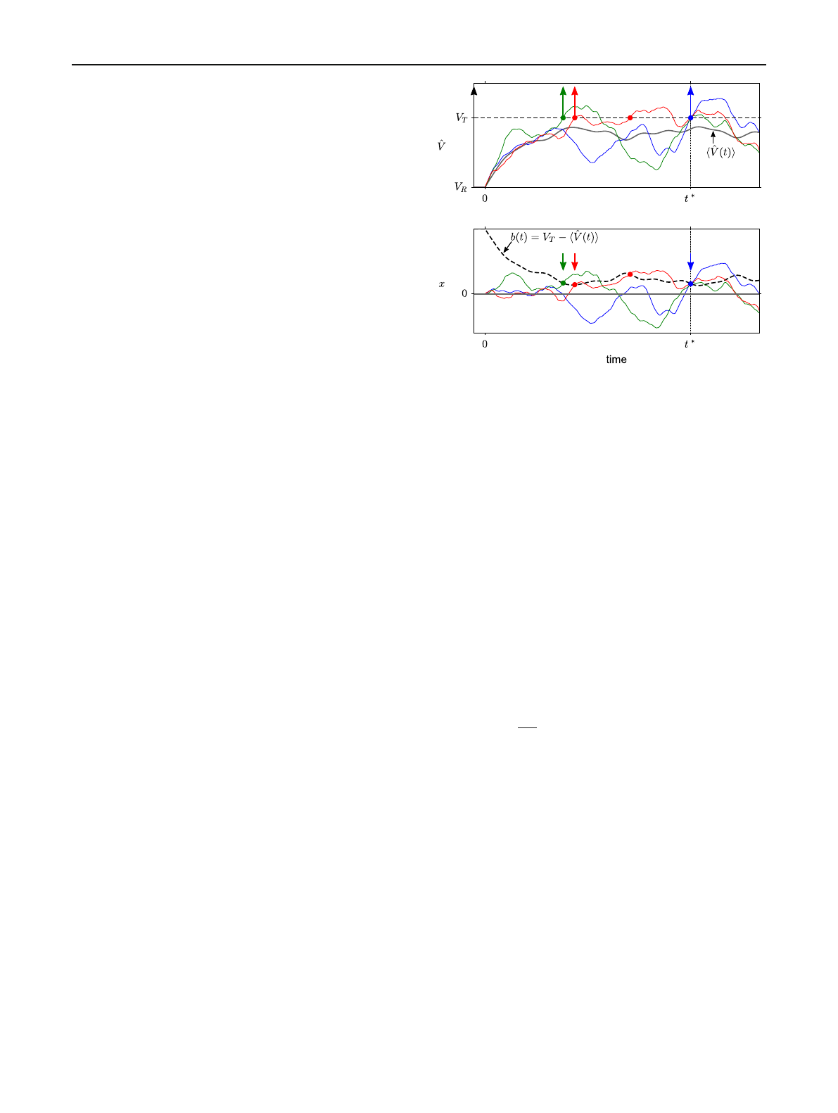
tics. The resulting non-resetting process ˆ

V(t)is the freely

evolving solution of Eq. (1) without reset and with initial

conditions ˆ

V(0)=VR,η(0)∼N(0,σ2

η)(Fig. 1a). This

non-resetting process will be useful for the level-crossing

approach below.

For mathematical convenience, we will now reformulate

the FPT problem in terms of a time-homogeneous process

x(t)and a moving boundary b(t), so as to eliminate the

time-dependent parameter μ(t)in Eq. (1) (Fig. 1b). This is

achieved by subtracting the mean non-resetting membrane

potential ˆ

V(t)=u(t):

(a)

(b)

Fig. 1 First-passage time of an integrate-and-fire neuron model and

an equivalent model with moving boundary. aAt time t=0, differ-

ent realizations of the non-resetting membrane potential ˆ

V(t)(colored

thin lines) are released from the reset potential VR. The non-resetting

membrane potential follows a Gaussian process with time-dependent

mean ˆ

V(t)(gray thick line). Shown are three realizations (green, red,

blue lines) that have an identical threshold crossing at time t=t∗

(blue circle), which is not necessarily the first crossing (indicated by an

arrow). bTransformation to an equivalent time-homogeneous process

x(t)with moving boundary b(t), in which the positions of thresh-

old crossings are preserved. Parameters: τs=4 ms, τm=10 ms,

σV:=σx(∞)=0.25(VT−VR)

x(t)=ˆ

V(t)−u(t)(3)

b(t)=VT−u(t), (4)

where u(t)is given by Eq. (2a) with initial condition u(0)=

VR. Furthermore, setting y=η/τm,γ=1/τm,τy=τsand

D=τsσ2

η/τ2

m, we find the Langevin equation

˙x=−γx+y(5a)

τy˙y=−y+√2Dξ(t)(5b)

with initial conditions

x(0)=0,y(0)∼N(0,σ2

y)(6)

The dynamics of x(t)can be interpreted as an overdamped

motion of Brownian particle in a parabolic potential sub-

ject to a colored noise y(t)(Ornstein–Uhlenbeck process).

Here, Dand τyare intensity and the correlation time of the

noise, respectively, and γis the friction coefficient. As before,

ξ(t)is a zero-mean Gaussian white noise. At time t=0,

the random initial condition for the colored noise ycorre-

sponds to a stationary Gaussian distribution with mean zero

and variance σ2

y=D/τy. By construction, the domain of

the particle is bounded from above by the time-dependent

123

Biological Cybernetics (2021) 115:539–562 543

boundary b(t), where b(0)>0 and b(t)is a differentiable

function of time. The FPT t∗is defined as the time when

x(t)exits the domain, i.e., when it reaches the boundary,

for the first time. The FPT density will be denoted by P(t),

i.e., P(t)dt=Prob(t∗∈[t,t+dt)) for an infinitesimal

time interval of length dt. We emphasize again that the FPT

density of the Brownian particle x(t)with moving boundary

b(t)is the same as the FPT density of the membrane potential

V(t)with respect to the constant threshold VT.

Beyond neuroscience, the escape of the doubly low-

pass filtered process, Eq. (5), from a domain with moving

boundary b(t)may serve as a simple archetypal model for

non-stationary FPT problems. One prominent example is

reaction times of bimolecular chemical reactions (Hänggi

et al. 1990). If x(t)is interpreted as a reaction coordinate and

the domain x<b(t)corresponds to the reactant state, the

boundary b(t)can be interpreted as a time-dependent energy

barrier that needs to be surpassed to reach the product state.

Accordingly, the first-passage time can be interpreted as the

reaction time.

3 Level-crossing theory for a moving barrier

3.1 Hazard-rate representation of first-passage-time

density

To find approximations to the FPT density from approxi-

mate hazard rates, we use concepts from renewal theory,

especially the notion of hazard rate and survival probabil-

ity (Cox 1962). Because the process Eq. (5) starts at time

0, the hazard rate λ(t)is defined here as the conditional

probability per small time interval dtto find a boundary

crossing in the interval (t,t+dt)given the absence of

crossings in the interval (0,t). On the other hand, the sur-

vival probability S(t)is defined as the probability of an

absence of crossings in (0,t). The two definitions imply that

S(t+dt)=S(t)(1−λ(t)dt), hence dS(t)/dt=−λ(t)S(t).

Because the survival probability is unity at time t=0, we

thus obtain S(t)=exp −t

0λ(s)dsfor t>0. The prob-

ability to find the first crossing after time 0 in the interval

(t,t+dt)is equal to the probability to find a crossing in

(t,t+dt)and to have no crossings in (0,t). Hence, the FPT

density is given by the product P(t)=λ(t)S(t),or

P(t)=λ(t)exp −t

λ(s)ds.(7)

Given the hazard rate λ(t)for t>0, Eq. (7) provides a

simple formula for the FPT density. An advantage of this

representation is that the exponential factor can be turned

into a first-order differential equation,

P(t)=λ(t)S(t), dS

dt=−λ(t)S(t), S(0)=1.(8)

Thus, if the hazard rate λ(t)can be efficiently computed

for t>0, this representation permits an efficient numeri-

cal integration of the first-passage-time density forward in

time. Therefore, the main strategy in this paper is to derive

computationally efficient approximations for the hazard rate.

In general, the calculation of the hazard rate is as difficult

as the calculation of the FPT density itself. However, finding

approximations for λ(t)has several advantages over direct

approximations of P(t). Firstly, as a probability density, P(t)

must satisfy the normalization to unity. Thus, the value of the

FPT density at different times cannot be calculated indepen-

dently. In particular, the value of P(t)strongly depends on

the values for t∈(0,t). By contrast, λ(t)is not a probability

density and can thus, in principle, be arbitrary as long as it

is nonnegative and S(t)=exp −t

0λ(s)dsconverges to

zero as t→∞. Thus, if we are able to find any approxi-

mation for λ(t), the normalization of P(t)is guaranteed by

Eq. (7).

Secondly, the character of the hazard rate is more local

in time than the FPT density, and thus, we expect more

efficient approximations for the hazard rate. The non-local

character of P(t)has been already mentioned above. More-

over, the non-locality becomes particularly evident by the

integral in Eq. (7), which accumulates the history of hazard

rates. The exponential factor S(t)shaped by this integral thus

contributes a trivial history-dependence of the FPT density

P(t), which is present already for time-homogeneous pro-

cesses. By contrast, this trivial history-dependence is divided

out in the hazard rate λ(t)=P(t)/S(t).Theremaining

time-dependence of the hazard rate singles out effects of

non-stationarity and explicit time-dependence of the system,

which can be captured by local variables. Thirdly, because

of the locality in time, time-dependent rates are interesting

in its own right as they are often the natural choice to model

escape processes in terms of a Markovian dynamics and mas-

ter equations.

From the above considerations, it becomes clear that the

hazard rate representation, Eq. (7), is only useful if we suc-

ceed to derive approximations for λ(t)that are local in time.

This means that we are seeking an approximation of the haz-

ardrateintheform

λ(t)≈Φb(t), ˙

b(t),...,{zi(t)},t,(9)

which may depend on time explicitly and through a few

variables such as the value and its derivative of the time-

dependent boundary, b(t)and ˙

b(t), respectively, and possibly

through a few auxiliary variables zi(t)that obey simple ordi-

nary differential equations. Note that we use the notations Φ

for the boundary-dependent hazard rate of the model Eq. (5)

123

Loading more pages...