
applied
sciences
Article
Three-Dimensional Mapping of Forest Soil Carbon Stocks
Using SCORPAN Modelling and Relative Depth Gradients in
the North-Eastern Lowlands of Germany
Alexander Russ 1,*, Winfried Riek 1,2 and Gerd Wessolek 3
Citation: Russ, A.; Riek, W.;
Wessolek, G. Three-Dimensional
Mapping of Forest Soil Carbon Stocks
Using SCORPAN Modelling and
Relative Depth Gradients in the
North-Eastern Lowlands
of Germany. Appl. Sci. 2021,11, 714.
https://doi.org/10.3390/app11020714
Received: 16 November 2020
Accepted: 5 January 2021
Published: 13 January 2021
Publisher’s Note: MDPI stays neu-
tral with regard to jurisdictional clai-
ms in published maps and institutio-
nal affiliations.
Copyright: © 2021 by the authors. Li-
censee MDPI, Basel, Switzerland.
This article is an open access article
distributed under the terms and con-
ditions of the Creative Commons At-
tribution (CC BY) license (https://
creativecommons.org/licenses/by/
4.0/).
1Landesbetrieb Forst Brandenburg, 16225 Eberswalde, Germany; W[email protected]
2Fachbereich für Wald und Umwelt, Hochschule für nachhaltige Entwicklung Eberswalde,
16225 Eberswalde, Germany
3Institut für Ökologie, Technische Universität Berlin, 10587 Berlin, Germany; Gerd.W[email protected]
*Correspondence: Alexander[email protected]
Abstract:
To cope with the challenges in forest management that are contemporarily caused by
climate change, data on current chemical and physical soil properties are more and more necessary.
For this purpose, we present a further amalgam of depth functions and SCORPAN modelling to
provide data at arbitrary depth layers. In this concept, regionalisation is split up into the modelling
of plot totals and the estimation of vertical distributions. The intended benefits by splitting up
are: consistency between estimates on plot level and depth layer level, avoidance of artificial depth
gradients, straightforward interpretation of covariates in the sense of pedogenetic processes, and
circumnavigation of the propagation of uncertainties associated with separation between horizons
during field sampling. The methodology was tailored to the circumstances within the north-eastern
lowlands and the utilisation of current inventory data of the National Forest Soil Inventory (NFSI)
in Brandenburg (Germany). Using the regionalisation of soil organic carbon (SOC) as an example,
the application is demonstrated and discussed in detail. The depth to groundwater table and terrain
parameters related to the catchment area were the main factors in SOC storage. The use of kriging
did not improve the model performance. The relative depth gradients of SOC were especially
distinguished by tree species composition and stand age. We suppose that interesting fields of
application may be found in scenario-based modelling of SOC and when SOC serves as a basis for
hydrological modelling.
Keywords:
depth functions; SCORPAN modelling; soil forming factors; forest soils; soil organic
carbon; regionalisation; north-eastern lowlands; forest site mapping; Brandenburg
1. Introduction
Nowadays, regional data on forest soil properties are increasingly demanded for
various questions concerning forest management practices, like tree species selection,
liming, harvest intensity, or the detection of risk areas. Thus, quantitative data related to
climate change and its site-specific drought effects, as well as data on current soil nutrient
status, are required to support decision-making.
Soil organic carbon (SOC) profoundly influences a soil’s cation exchange capacity
[
1
–
3
], which is a key feature for nutrient supply to trees. Soil texture, SOC , and the usually
tightly correlated bulk density [
4
–
6
] are the main factors controlling the soil hydraulic
properties [
7
–
9
]. Especially in the case of the mainly sandy textured soils of the north-
eastern lowlands, soil organic carbon strongly influences the spatial patterns of hydraulic
properties [
10
]. In addition to these well-understood principles, which are widely used
in modelling water and element budgets, SOC also affects the wettability of soils [
11
,
12
]
and, thus, the development of preferential flow paths [
13
]. Implications of preferential flow
paths are not limited to percolation and actual soil water storage [
14
], and may also include
feedback effects on local climate [15].
Appl. Sci. 2021,11, 714. https://doi.org/10.3390/app11020714 https://www.mdpi.com/journal/applsci

Appl. Sci. 2021,11, 714 2 of 28
Whereas in the glacial deposits of the north-eastern lowlands, soil texture is largely
predetermined by parent material, other soil forming factors, like groundwater, vegeta-
tion/forest management, and climate, also have to be taken into consideration for soil
organic carbon. In particular, due to the influence of groundwater and vegetation, the
temporal variation of SOC is expected to be high (compared to soil texture). Since en-
richment of soils with soil organic matter usually starts just after deposition of parent
material, tighter correlations with current terrain can also be expected. On the other hand,
to cope with the temporal variation, contemporary measurements of SOC are strictly
needed for regionalisation.
Over the last decades, several approaches for mapping SOC have been developed,
which generally make intense use of terrain parameters derived from digital elevation
models. Further covariates related to soil forming factors, like climate data, geological
mapping units, or data on landcover, are also frequently used. The methods usually
involved range from machine learning techniques, like support vector machines [
16
] or
artificial neural networks [
17
], to all kinds of statistical models, such as stepwise linear
regression and decision trees [
18
–
21
]. Especially since the introduction of the SCORPAN
framework for digital soil mapping by McBratney et al.
[22]
, which extended the classic
concept of soil forming factors [
23
] by soil and space, the additional use of geostatistics
in regionalisation approaches for SOC became a widely used technique [
24
]. Newer
approaches also use deep learning [
25
], data augmentation [
26
], and increment-averaged
kriging [27] to predict multiple depths with a single model.
The majority of studies conducted are on the prediction of SOC for predefined depths
of the entire soil solum or discrete soil layers. Prior to development of prediction models, it
is therefore necessary that the solum depth or soil layer boundaries are well defined for
the respective purposes. If the SOC of several soil layers should be mapped, fitting of the
increasing number of prediction models becomes more and more time consuming. The
SOC stock of every layer is then treated as unbounded random variables (see also [
28
]).
Thus, it becomes far from straightforward to ensure consistency between SOC stored in
single layers and the stocks of the entire soil solum at every single site in the resulting maps.
Analogous problems arise for the resulting depth gradients of SOC, which might
adopt artificial shapes. Furthermore, fitting of individual models for respective soil layers
forces the user to deal with several different estimates of variable importance. Except for
soil layers with a priori well-known differences regarding the main processes for carbon
enrichment, such as the organic layer and mineral soil, it will hardly be possible to logically
interpret the influence of covariates in terms of soil forming factors. This may hinder the
optimal selection of predictors and detection of spurious covariates to be excluded. Last
but not least, individual regionalisation of depth layers may enhance the propagation of
potentially large sampling errors caused by incorrect separation. Such errors especially
result from mingling of the organic layer and mineral soil [29].
The usage of depth functions to describe the vertical variation of soil properties
has a long tradition in soil science (see [
30
] for a detailed overview). The application of
soil attribute depth functions in three-dimensional spatial prediction of soil properties
was already proposed by Bishop et al.
[31]
. It has also already been shown that the
concept of depth functions is beneficial in mapping SOC distribution throughout the soil
profile: Equal-area quadratic smoothing splines were used to derive SOC for homogeneous
depth increments from legacy profile data as a data basis for the development of artificial
neural networks and regression models [
21
,
32
,
33
]. To obtain maps of continuous depth
functions, Malone et al.
[32]
utilised equal-area quadratic splines for interpolation through
predicted SOC contents of discrete soil layers after regionalisation. To calculate weighted
means of SOC for mapping units from available legacy soil data, Odgers et al.
[34]
applied
equal-area quadratic smoothing splines. From a more conceptual perspective, depth
functions are used for two reasons within 2.5D soil mapping frameworks [
35
]: The first
reason is the harmonisation of soil observations. Equal-area quadratic smoothing splines
are then often fitted to depth interval values after mapping to derive continuous depth
Appl. Sci. 2021,11, 714 3 of 28
functions for each pixel mapped. The equal-area smoothing splines of Bishop et al.
[31]
can
be considered as the state of the art for these two applications for one reason in particular:
The interpolation process preserves the masses originally measured or predicted on a depth
interval basis (especially for small values of λ).
Direct utilisations of depth functions during the mapping process itself are given
by Mishra et al.
[36]
and Kempen et al.
[37]
. Mishra et al.
[36]
used ordinary kriging to
interpolate parameters of exponential functions fitted to single-point observations before-
hand. Kempen et al.
[37]
predicted parameters of soil-type-specific depth functions of SOC
using cokriging.
By using relative depth gradients, we try to strengthen the interpretability of SCOR-
PAN factors in three-dimensional mapping of SOC in forest soils. Our further objectives
were to ensure the consistency between solum stocks and stocks within single depth layers,
to avoid the construction of artificial depth gradients, and to lessen the propagation of
sample separation errors. The basic conceptual hypothesis of the method is that distinguish-
ing between covariates that control horizontal and vertical distribution of SOC simplifies
variable selection during model development. Even though increasing interpretability may
decrease model performance measures, we believe that a good understanding of covariates
in terms of soil forming factors is valuable for the mapping results.
2. Material and Methods
For the regionalisation of SOC stocks in the north-eastern lowlands, we started with
the general methodology proposed by Kempen et al.
[37]
. The main accommodations to
the requirements for mapping SOC in the north-eastern lowlands concern a simplified
derivation of depth functions, which does not require expert-knowledge-based groupings
like horizons and soil types. Additionally, we tried to facilitate the accessibility of the
main factors controlling the horizontal and vertical distribution of SOC. To achieve this, we
substituted soil-type-specific depth functions with data-driven clustering and split up the
mapping process for the vertical and horizontal distribution of SOC with relative depth
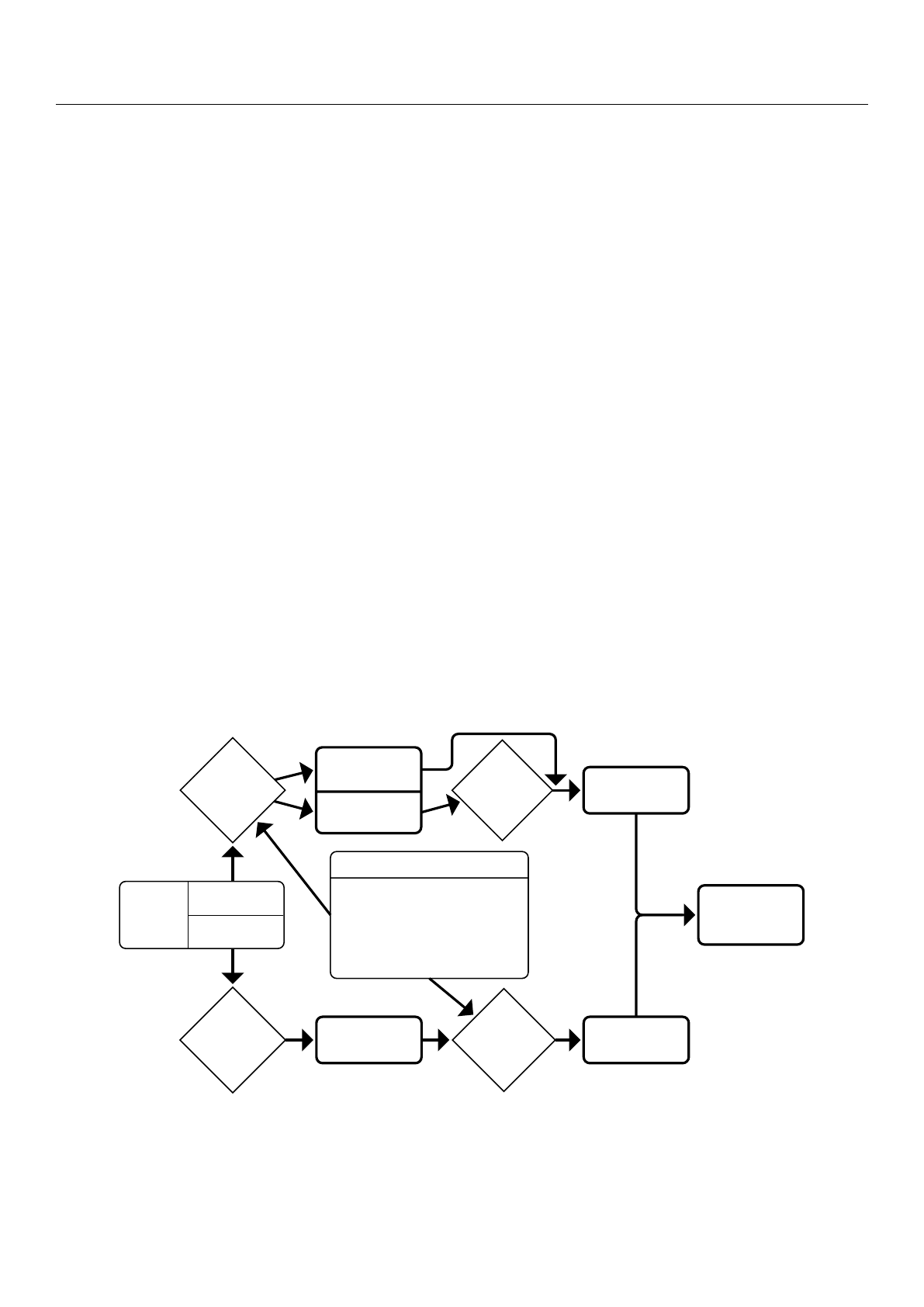
gradients. A flowchart of the methods and data involved is given in Figure 1.
SOC
inventory
data
solum stocks
depth layers
scorpan factors
S soil
C climate
O organisms land-use
R relief
P parent material
A age
N space
regression
analysis
pred. values
residuals
geostatistics
predicted
solum stocks
cluster
analysis
relative depth
gradients
classification
tree
depth gradient
type probability
predicted
SOC stocks in
depth layers
Figure 1.
Conceptual framework for mapping soil organic carbon (SOC) stocks in depth layers using SCORPAN modelling
and relative depth gradients.
In the first step, stepwise regression analysis was used to select the most significant
covariates, which determine whole solum SOC stocks at inventory plots, from a bundle of
potentially relevant SCORPAN factors. Afterwards, the residuals of the fitted regression

Appl. Sci. 2021,11, 714 4 of 28
models were examined using geostatistical methods (variogram analysis, ordinary kriging)
on spatial dependencies. Hence, the regionalisation of the SOC solum stocks complied
with the widely used regression kriging discussed in detail by Hengl et al. [38].
The regionalisation of depth gradients started with calculation of relative SOC stocks
within the particular depth layer by expressing single stocks in proportion to solum
stocks. The obtained relative depth gradients were then grouped into depth gradient
types using cluster analysis. Finally, classification tree approach was used to estimate the
probability that a site was in one of the distinct depth types. In addition to the purpose
of regionalisation, the resulting classification tree offers insights into the main factors
controlling the vertical distribution of SOC.
2.1. Inventory Data
To address the expected temporal variably of SOC adequately, we restricted the SOC
data invoked to inventory and inventory-like data. Our primary source of SOC data
was thus the second National Forest Soil Inventory (NFSI) [
39
]. An additional NFSI-like
soil sampling campaign was conducted at a regional scale to enhance the analysis of
topographic effects on SOC. Within the NFSI, field sampling was conducted during 2006
and 2009. At the regional scale, the collection of soil samples was done in the years 2008
and 2009 [
40
]. We did not make use of additional legacy profile data to avoid biased
estimates on total SOC stocks and to prevent a mix-up of spatial and temporal effects on
SOC. In contrast to the often-used legacy profile data, the NFSI comes with six well-defined
uniform depth layers (organic layer, 0–5, 5–10, 10–3, 30–60, and 60–90 cm). Hence, the
homogenisation or refinement of soil layers was not necessary prior to regionalisation. The
volumetric SOC contents (kg m
−3
) were obtained by using Equation (1), where
ρfe
,
Corg
,
and CF denote the bulk density of the fine earth (kg m
−3
), the concentration of organic
carbon (kg kg−1), and the volume fraction of coarse fragments (%), respectively.
SOC =ρfe Corg(1−CF
100)(1)
The volume fraction of coarse fragments was estimated in the field and measured by
sieve analysis in the laboratory (depending on rock size). Mass fractions obtained from the
sieve were transformed into volume fractions by assuming a rock density of 2.65gcm
−3
.
The bulk density of the fine earth was determined on soil-core samples. Mass and volume
fractions of coarse fragments (>2 mm) contained within the core samples were excluded
from the calculation. Organic carbon was determined by dry combustion using a total
analyser (LECO CNS-2000). All laboratory analyses were performed in compliance with
the NFSI standards, which are documented in detail in GAFA [41].
2.2. Environmental Covariates
Since the preliminary considerations strongly suggested that SOC is controlled by a
wide range of influences, we tried to obtain environmental covariates that address all seven
SCORPAN factors appropriately. A short overview of the compiled variables is given in
Tables 1and 2.
Covariates related to parent material and soil properties were primarily derived from
forest site mapping data [
42
,
43
] and by means of digital soil mapping techniques [
40
,
44
].
In addition to widely used particle size fractions, we additionally computed the geometric
mean particle size Dg%
...
for numerical characterisation of the soil texture. Dg%
...
was
originally proposed by Meersmans et al.
[45]
to improve the reflection of SOC variation
due to texture. For estimates of the depth of groundwater, we additionally considered
water-table maps based on monitoring wells [46].
Climatic factors were directly taken from the detailed compilation by Riek et al.
[47]
.
The selection of indicators to be considered was guided by assumptions on dominant
processes influencing the storage of SOC inside the study area. Thus, CWB
win
(climatic
water balance during winter) and P
win
(winter precipitation) were chosen as proxies for

Appl. Sci. 2021,11, 714 5 of 28
vertical translocation, whereas CWB
sum
(climatic water balance in the summer half-year),
P
sum
(summer precipitation), and
Ta
(annual mean temperature) were used to indicate
climatic effects on soil biological activity. Additionally, we calculated the annual rage
of temperature
∆T
as a surrogate for continentality and the number of frost-free days.
The latter was originally introduced by Ramann
[48]
and then revisited by Jenny
[23]
as
Ramann’s Weathering Factor, expressing the length of the ‘chemical weathering season’.
Table 1. Environmental covariates for the regionalisation of SOC arranged by the associated SCORPAN factors.
Soil Properties (s), Parent Material (p)
CF... coarse fragments [%]
S%...,Si%...,C%...
proportions of particle-size
classes (sand, silt, clay)
Dg%... geometric mean particle size
zCaCO3depth of calcareous horizon
zGW depth of groundwater
Climate (c)
CWBsum,CWBwin climatic water balance (seasonal)
Taannual mean temperature
nd>0◦Cfrost-free days
∆T
annual range of temperature (as
surrogate for continentality)
Pa,Pwin,Psum precipitation (annual, seasonal)
Organisms, Vegetation, Land Use (o)
p
deciduous
,p
pine
,
pbeech,poak proportions of tree species
Topography (r)
terrain attributes derived from the digital elevation
model (DEM) (see Table 2)
Age (a)
series...
geochemical series (age of de-
posit)
tstand, forest stand age
Spatial Position (n)
WA200
,
WA500
,
WA1000,
proportion of surrounding forest
area (within search radii of 200,
500, 1000m)
ledge distance to nearest forest edge
The proportions of tree species were derived from forest inventory data (‘Datenspei-
cher Wald’) to obtain forest-specific indicators on land-use effects. The usage of forest
inventory data allowed us to calculate the respective percentages from ratios of a single-
species basal area to the total basal area of the forest stands. In the rare case of missing
data, CORINE landcover classes [49] were used instead (applies to mapping only).
The role of topography on SOC was examined with several terrain attributes derived
from a digital elevation model (DEM). As the cell size of the underlying DEM was 25m,
the terrain attributes derived form the environmental covariates with the highest spatial
resolution in our study. Seeing that the covariates derived from DEM might be able to
improve the prediction of SOC at the smallest spatial scales and the general availability of
DEM data, we made exhaustive use of them. Nevertheless, the selection of indices from the
vast number of existing terrain attributes was once again strictly constrained with respect
to the theory of topography as a soil forming factor. The computed terrain attributes are
tabulated in Table 2.
The time factor on SOC was considered from a geologic and a forest management
perspective. For this, we computed the mean stand age as a basal-area-weighted average
on the basis of forest inventory data. To cope with the problem of soil formation time, we
used the geochemical series gathered by forest site mapping as a rough estimate.
Loading more pages...