
Oscillatory Source Tensor Discriminant Analysis (OSTDA): A regularized
tensor pipeline for SSVEP-based BCI systems
Tania Jorajuría
a,b,1,2
, Mina Jamshidi Idaji
b,c,d,2
, Zafer _
Isßcan
e
, Marisol Gómez
a
, Vadim V. Nikulin
b,f,
⇑
,3
,
Carmen Vidaurre
a,
⇑
,3
a
Department of Statistics, Computer Science and Mathematics, Universidad Pública de Navarra, Pamplona, Spain
b
Department of Neurology, Max Planck Institute for Human Cognitive and Brain Sciences, Leipzig, Germany
c
International Max Planck Research School NeuroCom, Leipzig, Germany
d
Machine Learning Group, Technical University of Berlin, Berlin, Germany
e
Department of Electrical & Electronics Engineering, Faculty of Engineering and Natural Sciences, Bahcesehir University, Istanbul, Turkey
f
Centre for Cognition and Decision Making, Institute for Cognitive Neuroscience, National Research University Higher School of Economics, Russian Federation
article info
Article history:
Received 26 February 2021
Revised 28 May 2021
Accepted 25 July 2021
Available online 23 December 2021
Communicated by Zidong Wang
Keywords:
Brain-computer interface
Steady-state visual evoked potential
Spatio-spectral decomposition
Higher order discriminant analysis
Analytical regularization
Tensor-based feature reduction
abstract
Periodic signals called Steady-State Visual Evoked Potentials (SSVEP) are elicited in the brain by flickering
stimuli. They are usually detected by means of regression techniques that need relatively long trial
lengths to provide feedback and/or sufficient number of calibration trials to be reliably estimated in
the context of brain-computer interface (BCI). Thus, for BCI systems designed to operate with SSVEP sig-
nals, reliability is achieved at the expense of speed or extra recording time. Furthermore, regardless of the
trial length, calibration free regression-based methods have been shown to suffer from significant perfor-
mance drops when cognitive perturbations are present affecting the attention to the flickering stimuli. In
this study we present a novel technique called Oscillatory Source Tensor Discriminant Analysis (OSTDA)
that extracts oscillatory sources and classifies them using the newly developed tensor-based discriminant
analysis with shrinkage. The proposed approach is robust for small sample size settings where only a few
calibration trials are available. Besides, it works well with both low- and high-number-of-channel set-
tings, using trials as short as one second. OSTDA performs similarly or significantly better than other
three benchmarked state-of-the-art techniques under different experimental settings, including those
with cognitive disturbances (i.e. four datasets with control, listening, speaking and thinking conditions).
Overall, in this paper we show that OSTDA is the only pipeline among all the studied ones that can
achieve optimal results in all analyzed conditions.
Ó2021 The Authors. Published by Elsevier B.V. This is an open access article under the CC BY-NC-ND
license (http://creativecommons.org/licenses/by-nc-nd/4.0/).
1. Introduction
A Brain-Computer Interface (BCI) is a system that uses brain sig-
nals to deliver commands according to their decoding [1]. Its appli-
cations range from neurological rehabilitation [2–6] to
communication for disabled people [1,7], controlling external
devices [8,9], marketing [10] and entertainment [11]. Over the past
years, several BCI systems have been developed using different
electroencephalogram (EEG) brain responses, including sensorimo-
tor rhythms [12–18], event-related potentials [19,20] and visual-
evoked potentials [21–25]. Among them, Steady-State Visual
Evoked Potentials (SSVEP) have attracted attention due to their
high signal-to-noise ratio (SNR) [26], robustness [27] and greater
information transfer rate [28,29], when compared to other brain
responses.
SSVEP signals are generated when a subject is looking at a flick-
ering stimulus. As a response, periodic signals with fundamental
frequency equal to the stimulus frequency, together with its har-
monics, can be observed in the occipito-parietal regions [30]. Based
on this phenomenon, the SSVEP-based BCIs can differentiate the
brain response to stimuli with different flickering frequencies
(classes) and therefore generate a specific output for each of those
classes. In order to analyze SSVEP signals, several methodologies
have been used in the recent years. Some of them include fast
Fourier transform [31,32], power spectral density-based analysis
[33–36], common spatial patterns [37], minimum energy combina-
tion [27,38,39], multivariate linear regression [40] and linear dis-
https://doi.org/10.1016/j.neucom.2021.07.103
0925-2312/Ó2021 The Authors. Published by Elsevier B.V.
This is an open access article under the CC BY-NC-ND license (http://creativecommons.org/licenses/by-nc-nd/4.0/).
⇑
Corresponding authors.
ra.es (C. Vidaurre).
1
Present address.
2
Both authors contributed equally.
3
Both senior authors contributed equally.
Neurocomputing 492 (2022) 664–675
Contents lists available at ScienceDirect
Neurocomputing
journal homepage: www.elsevier.com/locate/neucom
criminant analysis [41], among others. However, the most popular
method in the literature is the Canonical Correlation Analysis (CCA)
[42,43,39,44,45] and its extensions [46–48] or combinations with
other methods [49]. CCA-based methods aim at finding spatial fil-
ters that maximize the correlation between SSVEP signals and
sine–cosine reference templates at the fundamental and harmonic
frequencies of the stimuli. Many CCA-based methods have the
advantage of not requiring calibration (training) data, thus reduc-
ing or even eliminating the need of performing extra-recordings.
Nevertheless, they do not consider the possibly high overlap
between different classes and are very sensitive to cognitive per-
turbations that can be present in out-of-the-lab environments
[50]. Recently, a new method called Task-Related Component Anal-
ysis (TRCA) [51,52] has been developed in order to reduce trial
length in the design of SSVEP-based BCIs and operate at higher
speeds. This method is based on the maximization of the inter-
trial covariance matrix, and it was shown to be significantly more
efficient than CCA under time restricting conditions such as short
trial lengths. Another state-of-the-art method developed for
high-speed SSVEP-based BCIs, which we will refer to as High-
Speed BCI (HSBCI), was presented in [28]. HSBCI decomposes
SSVEPs and template signals into sub-band components by apply-
ing a filter bank analysis, and employs CCA-based spatial filters to
extract correlation features. Both TRCA and HSBCI use calibration
data to train their corresponding feature extraction procedures.
In fact, feature training has proven to critically increase SSVEP-
based BCI performance [53]. TRCA and HSBCI methods were origi-
nally introduced for a set of pre-selected channels over parietal and
occipital areas. Even though they both achieve high accuracy
results with short trial lengths, their ability to accurately classify
SSVEP data in the small sample size and in settings with higher
number of channels has to be established yet. Besides, in this
manuscript we also study how cognitive perturbations affect the
aforementioned state-of-the art methods to understand how they
could work in out-of-the-lab environments.
In this paper we propose a novel analysis pipeline, namely
Oscillatory Source Tensor Discriminant Analysis (OSTDA), to
extract SSVEP features from EEG data. Within this pipeline, we
introduce a method called shrinkage higher order discriminant
analysis (sHODA). sHODA is a modification of higher order discrim-
inant analysis (HODA) [54] that includes an analytic shrinkage
inspired by [55] as a tool for overcoming the small sample size
problem. sHODA is then used to extract features from oscillatory
brain sources, resulting in high accuracy results with trial lengths
as short as one second. In this manuscript, we compare OSTDA to
the aforementioned TRCA, HSBCI and CCA methods, and show that
it has the benefits of all of them, but none of their disadvantages. In
particular, we demonstrate that OSTDA is more robust in the small
sample size setting, and less affected by perturbations. Moreover,
our pipeline performs well with few channels and also in settings
with a high number of channels, which is a required condition in
certain applications. Thus, in this manuscript we propose a practi-
cal and fast SSVEP-based BCI system.
The paper is organized as follows: we introduce our proposed
pipeline, OSTDA, in Section 2. There, we also present sHODA and
show the details of the comparison between OSTDA and state-of-
the-art methods. In Section 3we describe the experimental data
used in this study as well as the evaluation settings. In Section 4,
we explain the details about OSTDA parameter selection, and in
Section 5we detail the statistical analysis done. Section 6is dedi-
cated to analyze results, which are discussed in Section 7. Finally,
Section 8includes a brief conclusion of the paper.
2. Methods
2.1. Notation
In this manuscript, tensors are denoted by calligraphic letters
(e.g. X), matrices are denoted by boldface capital letters (e.g. X),
whereas boldface lower-case letters are used to denote vectors
(e.g. x), and regular letters for scalars (e.g. x).
We denote the data matrix of the k-th training trial as
X
ðkÞ
2R
CT
, where Cis the number of channels and Tis the number
of time samples. Therefore, the training data with Ktrials is a
three-way tensor X2R
CTK
.
2.2. Oscillatory Source Tensor Discriminant Analysis (OSTDA)
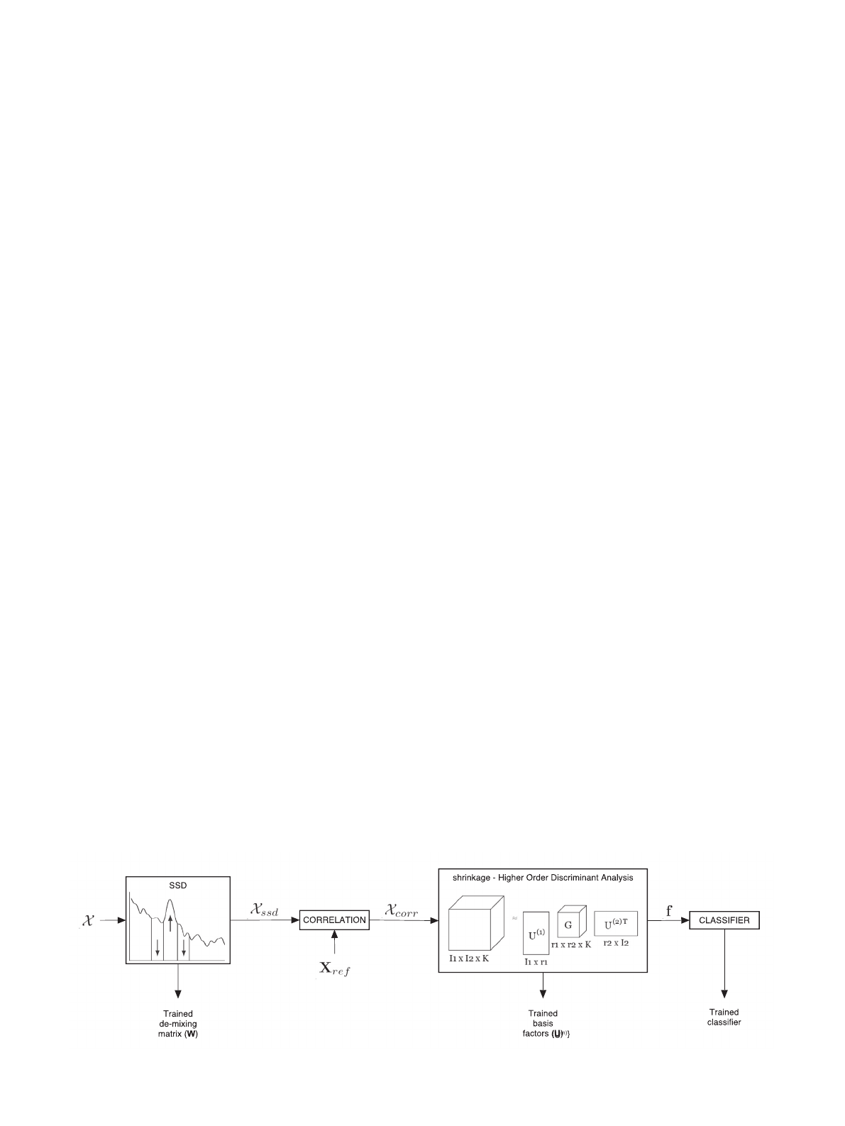
Fig. 1 shows the block diagram of our proposed feature extrac-
tion and classification pipeline, named Oscillatory Source Tensor
Discriminant Analysis (OSTDA). In the following sections, we elab-
orate upon the details necessary to employ OSTDA.
2.2.1. Feature extraction
Spatio-Spectral Decomposition (SSD). SSD [56] is a multivariate
and unsupervised method that aims at separating oscillatory
sources from brain signals recorded with multiple electrodes by
maximizing their signal-to-noise ratio (SNR) at the frequency band
of interest. It computes spatial filters that are basis vectors of a
subspace where the ratio of the signal power in a specific fre-
quency band to the power of signals at its marginal bands is
maximized.
Assume that the measured signal is X¼SþN, with Scorre-
sponding to the signal-of-interest in a specific frequency band
and Nthe noise component in a broad band. While filtering Xin
the frequency band of interest (resulting in X
s
) gives an approxi-
mation of the signal-of-interest plus noise, filtering in two narrow
bands (1 to 2 Hz) around the frequency band of interest (resulting
in X
n
) approximates the noise alone. Using generalized eigenvalue
Fig. 1. The block diagram of our proposed pipeline, OSTDA.
T. Jorajuría, M. Jamshidi Idaji, Z. _
Isßcan et al. Neurocomputing 492 (2022) 664–675
665

decomposition, SSD finds the optimum spatial filter w2R
C1
that
maximizes the ratio
w
T
C
s
w
w
T
C
n
w
, where C
s
¼
1
T
X
s
X
T
s
and C
n
¼
1
T
X
n
X
T
n
.
In order to apply SSD to our data, we concatenated all the trials
of the training tensor X2R
CTK
to have a X2R
CTK
data matrix.
Then, we applied SSD on a broad-band range between ½5;32Hz.
This band was selected because it covers all the fundamental and
second harmonic frequencies of the flickering stimuli. Afterwards,
we selected n
SSD
sources (n
SSD
6C) from the SSD components. We
obtained the SSD spatial filters separately for each subject using
the training trials. We denote the SSD spatial filters by
W2R
Cn
SSD
. The projection of Xonto the SSD subspace is denoted
by X
ssd
2R
n
SSD
TK
, that corresponds to brain sources with
improved SNR within the frequency band ½5;32Hz.
Correlation with reference signals. As discussed before, a flick-
ering stimulus elicits brain activities oscillating with the funda-
mental frequency equal to the flickering frequency. Therefore,
one of the most informative SSVEP features is the similarity of
the EEG with single-tone sines and cosines at each flickering fre-
quency and its corresponding higher harmonics. In the case of this
study, there are four classes and we use the information of first and
second harmonics (similar to [50]). Thus, a total of M¼16 refer-
ence signals are necessary. In order to extract these similarities
and to reduce the dimensionality of the features, we computed
the Pearson’s correlation of each SSD source signal with these ref-
erence signals grouped in X
ref
2R
MT
. This resulted in the training
data tensor X
corr
2R
n
SSD
MK
, which is a concatenation of feature
matrices of all trials fX
ðkÞ
corr
g
K
k¼1
R
n
SSD
M
. In the following, we refer
to these feature matrices as correlation feature matrices.
Shrinkage Higher Order Discriminant Analysis (sHODA).
Higher Order Discriminant Analysis (HODA) [54], initially intro-
duced as DATER [57], is a generalization of linear discriminant
analysis (LDA) [58] for tensor data X
k
R
I
1
I
2
I
N
. In the special
case of matrix data, which is also the case of this manuscript,
assume fX
k
g
K
k¼1
R
I
1
I
2
is the set of the training data points cate-
gorized in multiple classes. In order to find the discriminant sub-
space for this data, a simultaneous matrix factorization should be
performed as the following [59]:
X
k
U
ð1Þ
G
k
U
ð2Þ
T
;k¼1;;Kð1Þ
The orthogonal basis factors fU
ðnÞ
2R
I
n
r
n
g
2
n¼1
are computed,
with the same idea as in LDA, by maximizing between-class covari-
ance of the projections and minimizing the within-class covari-
ance. The projections of data points (or the features) are
computed as:
G
k
¼U
ð1Þ
T
X
k
U
ð2Þ
ð2Þ
which can be vectorized and used for training a classifier. Test data
can be projected onto this discriminant subspace by using Eq. 2.
Note that G
k
2R
r
1
r
2
. Since r
n
<I
n
;n¼1;2, the discriminant sub-
space has a lower dimension than the original subspace of the data.
HODA employs an alternating least squares (ALS) algorithmic
scheme that iterates over the dimensions of the data tensor (here
the first two dimensions). In each iteration scatter matrices are
computed and the basis factors are estimated using an eigenvalue
decomposition. In other words, each iteration of the ALS algorithm
is an LDA problem as the following:
U
ðnÞ
¼argmax
U
ðnÞ
tr U
ðnÞT
S
n
b
U
ðnÞ
tr U
ðnÞT
S
n
t
U
ðnÞ
;s:t:U
ðnÞT
U
ðnÞ
¼Ið3Þ
where S
n
b
and S
n
t
are the between-class and total scatter matrices
of the n-th mode of the data tensor. In our special case of matrix
data, n¼1;2. More details about the computation of the scatter
matrices are presented in appendix A.
Tensor-based feature extraction methods are known to cope
well with small sample size scenarios [60,54]. However, even these
methods suffer from ill-conditioned scatter matrices. Therefore,
similar to conventional LDA, it is suggested that the within-class
covariance matrix should be regularized [54]. Previous works
[54,61] have implemented this regularization by means of a con-
stant regularization parameter. However, as we know from the lit-
erature on EEG classification, LDA can benefit from shrinkage,
where the shrinkage parameter is computed analytically in a
data-driven manner [55,62,63]. Inspired by [55], we implemented
an analytic shrinkage in HODA, and called it shrinkage-HODA
(sHODA), where the total scatter matrix of Eq. 3is regularized in
each of the iterations of the ALS algorithm. The optimization prob-
lem of sHODA is formulated as the following:
U
ðnÞ
¼argmax
U
ðnÞ
tr½U
ðnÞT
S
n
b
U
ðnÞ
tr½U
ðnÞT
ðS
n
t
þ
c
ðnÞ
IÞU
ðnÞ
;s:t:U
ðnÞT
U
ðnÞ
¼Ið4Þ
where c
ðnÞ
is the regularization parameter of mode n. sHODA com-
putes this regularization parameter of each mode in a data-driven
approach. As mentioned before, [54,61] have introduced a constant
regularization parameter to the total scatter matrix, i.e.
c
ðnÞ
¼c
0
¼const;8n. The constant regularization adds a challenge
of selecting this parameter as a hyper-parameter of the pipeline,
which makes the calibration phase computationally more expen-
sive. Additionally, a constant regularization parameter may not be
the optimum value for regularizing the LDA problem in all itera-
tions of the ALS algorithm. sHODA overcomes both of these draw-
backs and can improve the performance of the feature extraction
in small sample size scenarios. Additionally, data-driven computa-
tion of the shrinkage parameter eliminates one parameter from
the cross-validation parameter tuning. For the details about the for-
mulation and algorithm of sHODA, we refer the reader to appendix
A of this manuscript.
After applying sHODA on the correlation features of SSVEP data
(i.e. fX
ðkÞ
corr
g
K
k¼1
R
n
SSD
M
), the feature matrix f2R
Kr
1
r
2
is obtained
and used for classification. Note that the only parameters of sHODA
are the new dimensions of the feature space, i.e. R¼½r
1
;r
2
.
2.2.2. Classification
As in the original paper describing and analysing the datasets
used here [50], we applied the K-Nearest Neighbor (KNN) classifier
with five neighbors for all the analyses performed in this paper
with the OSTDA pipeline. The KNN implementation of the Statistics
and Machine Learning Toolbox of MATLAB
Ò
was used.
2.3. Benchmarking
We compared our proposed pipeline, OSTDA, with the following
state-of-the art methods.
Canonical Correlation Analysis (CCA). CCA is probably the most
popular method for feature extraction in SSVEP-based BCIs
[42,43,39,44,45]. CCA solves an optimization problem to find linear
mappings that maximize the correlation of two matrices. Here,
these two matrices are the EEG data from multiple electrodes
and the reference signals. In [50], for each SSVEP flickering fre-
quency, two sine–cosine reference signal matrices were used to
calculate canonical correlations; one of these matrices corre-
sponded to the stimulation frequency and the other one to its sec-
ond harmonic. Therefore, four canonical correlation values (CCA
features) were computed for each class, resulting in sixteen CCA
features.
To implement the above-mentioned CCA-based feature extrac-
tion in this paper, each trial was first detrended and band-pass fil-
T. Jorajuría, M. Jamshidi Idaji, Z. _
Isßcan et al. Neurocomputing 492 (2022) 664–675
666

tered between ½0:53;40Hz. This step removes DC, high frequency
artifacts and the 50 Hz power line noise [50]. Afterwards, the six-
teen CCA features were computed for each trial and classified with
a KNN classifier with five neighbors. This classifier achieved the
best classification results in the testing dataset in [50].
Task-Related Component Analysis (TRCA). TRCA [51] is a
recently published algorithm applied to high-speed SSVEP-based
BCIs. This method finds spatial filters that maximize the inter-
trial covariance matrix of each class separately by means of a gen-
eralized eigenvalue decomposition (more details can be found in
[52]).
In this paper, we followed the procedure explained in [51] to
implement TRCA, where the SSVEP signals are filtered into sub-
band components by using a filter bank. In order to fit the param-
eters of that work to the data used in this manuscript, the lowest
cut-off frequency was set to 5 Hz, thus we could include the small-
est flickering frequency. We computed the ensemble spatial filters
and the averaged templates for each stimuli and sub-band with the
training trials.
High-Speed BCI (HSBCI). A new high-speed SSVEP-based BCI
was introduced in [28]. HSBCI consists on a filter bank analysis that
decomposes SSVEPs and template signals into sub-band compo-
nents to extract correlation features using CCA-based spatial filters.
We calculated the SSVEP template signals with the training trials.
In order to implement HSBCI, we followed the procedure
explained in [28] with some exceptions to adapt the method to
the data analyzed here: the reference signals matrix to compute
CCA included the first and second harmonics, so the total fre-
quency range was ½5;32Hz. As for TRCA, we also set the lowest
cut-off frequency to 5 Hz to include the smallest flickering
frequency.
3. Experimental data
3.1. Data description
In this paper, we analyzed a public EEG dataset of a SSVEP-
based BCI recorded from 24 subjects from [50]. All subjects partic-
ipated in the study after giving a written informed consent in
accordance with the declaration of Helsinki and the experiments
were approved by the local ethics committee of National Research
University Higher School of Economics, Moscow [50]. The visual
stimuli consisted of four circles placed in different locations of a
screen, flickering at distinct frequencies of 5.45 Hz, 8.57 Hz,
12 Hz, and 15 Hz. Frequencies multiples of each other were
avoided in order to prevent coincidences between frequencies of
flickering stimuli and their higher harmonics. For more details
about the experimental setup, we refer the reader to [50].
Participants underwent offline and online (with feedback)
recording sessions. In this study, we used the offline data as the
training dataset and the online data as the testing dataset.
The offline session consisted of four runs of 25 trials each, with
a total of 100 trials (25 trials per class). In each offline trial, the sub-
jects were asked to focus on a randomly selected flickering circle
surrounded by a red oval for three seconds, followed by a one-
second resting period. In the online session, the subjects freely
chose a flickering circle to focus on for three seconds. After each
trial, the classification result was presented to the subject as a
feedback and they had to confirm or reject the result using the key-
board. There were four conditions (with and without perturbation)
in the online session (100 trials each, per subject). During each
condition, the subjects were asked to perform randomly one of
the following tasks, while looking at the stimulus: control (no per-
turbation), speaking (counting loudly and repeatedly from one to
ten), thinking (counting silently from one to ten repeatedly), and
listening (paying attention to a pre-recorded audio file where the
participant had counted from one to ten repeatedly).
EEG data were recorded from 60 channels based on the interna-
tional 10–20 system, as in Fig. 2, with the reference electrode on
the left mastoid and 1 kHz sampling rate. The data were segmented
using the stimuli markers specifying the onset and end of the flick-
ering. As aforementioned, offline and online trials of the studied
datasets were three seconds long. However, long trials decrease
the speed of BCI systems, thus an effort must be done to obtain
reliable results with short trial lengths. Consequently, in this study
we focused on short trials of only one second, with the aim of
increasing the information transfer rate of our system.
3.2. Evaluation settings
We evaluated the performance of two different settings with
our proposed pipeline and with the selected state-of-the-art meth-
ods. In particular, we analyzed how the training sample size and
the number of channels affect the performance of the studied
methods. The factor ‘‘sample size” addresses the amount of data
that is necessary to obtain a reliable performance. Reducing the
need of training (also called calibration) data, increases the ease
of use of BCIs. Typically, recording offline data is challenging
because participants become tired before starting the actual feed-
back BCI session. This problem is even greater for patients, whose
attention span might be compromised. Thus, BCI researchers inves-
tigate how short the training sessions can be to still obtain reliable
online performances [64–66], as we do in this work. On the other
hand, the factor ‘‘number of channels” is related to the trade-off
between a fast and easy setup with a low number of dimensions
and the need of flexible paradigms, specially in the case of partic-
ipants with special needs, for example due to pathologies of the
nervous system. This means that, specially for the case of patients,
it is not always possible to select only a few optimal channels, and
hence flexible systems with a higher number of dimensions might
be necessary. Thus, in order to design BCI systems that can be used
in out-of-the-lab conditions, it is necessary to study how reliable
they are under low sample size settings and with higher number
of dimensions, as we do here. That is, it is necessary to analyze
the trade-off between number of channels and the amount of avail-
able training data.
Sample size. Small sample size (SSS) problems in classification
arise when there are not enough training data points in compar-
ison to the number of unkowns. This condition results in overfit-
ting of the machine learning methods and therefore, a significant
drop in the classification results of test data is observed. In order
to assess the performance of our pipeline and other state-of-the-
art methods in SSS settings, we computed the classification results
for two numbers of training trials values. In particular, we used
only the first 5 or 25 trials of each class from the training dataset
for training. We refer to the case of using all the available training
data (i.e. 25 trials per class) as the full sample size (FSS) setting.
Fig. 2. Scalp plot of the electrodes configurations used in this study. 60-channel
setting: all shown electrodes; 9-channel setting: bold-circled electrodes.
T. Jorajuría, M. Jamshidi Idaji, Z. _
Isßcan et al. Neurocomputing 492 (2022) 664–675
667
Note that there are four classes and therefore we have in total 100
trials to train in FSS setting and 20 in the SSS setting.
Number of channels. We evaluated two different settings
regarding the number of channels used. The first setting included
all 60 EEG channels (all electrodes shown in Fig. 2). For the second
setting, only nine channels located in parietal and occipital areas
(bold-circled electrodes in Fig. 2) were selected according to
[28,51]. These channels are known to provide very good perfor-
mance for steady-state visual evoked potential paradigms [67].
4. Parameter selection
OSTDA pipeline has two parameters that were subject-
specifically selected: n
SSD
(the number of SSD components that
are retained) and R¼½r
1
;r
2
(the number of components retained
by sHODA in each mode).
The range of n
SSD
was determined based on the number of chan-
nels used [68]. For the 9-channel setting 5 6n
SSD
69, while for the
60-channel setting 10 6n
SSD
635.
Rwas restricted to a specific set of possible values based on the
resulting total number of features (equal to the product of the two
elements of vector R, i.e. r
1
r
2
) according to the following criteria:
as we have four SSVEP flickering frequencies (classes), the lower
limit was set to three; additionally, taking into account that the
total number of trials in the FSS is 100, the upper bound was lim-
ited to about a 10% of this value [69], in this case to 12. Thus, we
had 3 6r
1
r
2
612. Therefore, the resulting possible values for R
were: ½1;3;½1;4;½1;5;½1;6;½1;7;½1;8;½1;9;½1;10;½1;11;½1;12;
½2;2;½2;3;½2;4;½2;5;½2;6;½3;1;½3;2;½3;3;½3;4;½4;1;½4;2;½4;3;
½5;1;½5;2;½6;1;½6;2;½7;1;½8;1;½9;1;½10;1;½11;1;½12;1.
Among these values, the ones that satisfied r
1
6n
SSD
were used for
each n
SSD
.
For each evaluation setting, we selected n
SSD
and Rfor each sub-
ject based on the eigenvalues obtained in sHODA, taking the com-
bination of these two parameters that maximized the explained
percentage of variance. This was done with a chronological hold-
out cross-validation using the corresponding training dataset in
each sample size setting, taking the last 40% trials of each class
as the validation set. With these subject-specific parameters,
OSTDA was trained with all available trials in each sample size
setting.
5. Statistical Analysis
Two 3-way repeated measures ANOVA were applied to the clas-
sification results obtained with the testing dataset to see the influ-
ence of the analysis approach (OSTDA, TRCA, HSBCI, CCA), number
of training trials per class (5;25) and perturbation (Control, Listen-
ing, Speaking, Thinking) factors. They were performed separately
for individual accuracy values obtained with the 9- and 60-
channel settings, respectively.
For each ANOVA, we analyzed the sphericity of the response
variables in the repeated measures model, using a Mauchly’s test.
In case of rejection, we report the Greenhouse-Geisser adjusted
p-values. Furthermore, after each ANOVA we performed post hoc
tests using Tuckey’s honestly significant difference (HSD), when
the interaction of main factors was significant.
6. Results
6.1. Parameter selection (training dataset)
As mentioned in Section 4, we performed a chronological hold-
out to tune the parameters of OSTDA (n
SSD
and R) for each subject.
The last 40%trials of each class of the corresponding training data
were used as the validation set. Thus, subject-dependent parame-
ters were selected in each of the evaluation settings, i.e. 9- and
60-channel as well as small and full sample size (refer to
Section 3.2).
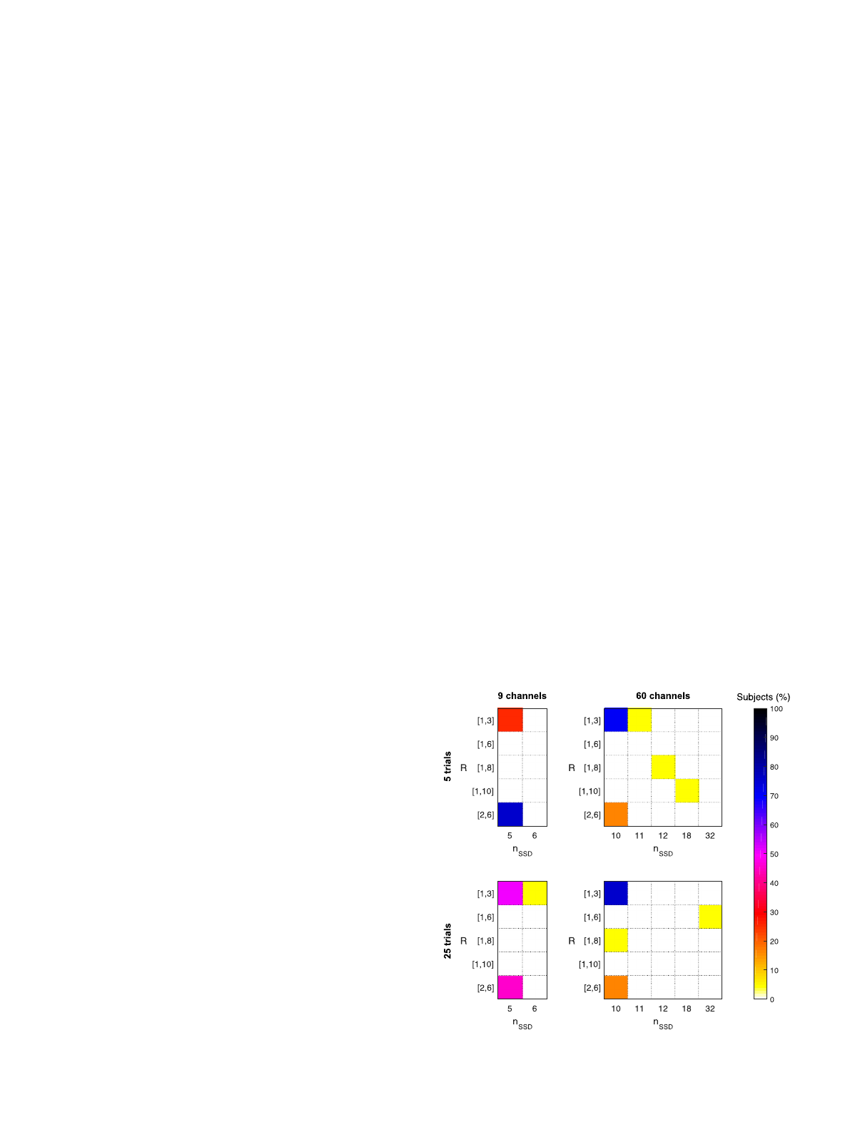
Fig. 3 shows the joint distribution of the selected parameters,
fn
SSD
;Rg, over all the subjects in each setting. In the 9-channel set-
ting the best parameters for most of the subjects are f5;½2;6g in
the SSS setting, selected for 75%of subjects, and f5;½1;3g and
f5;½2;6g in the FSS setting, selected for 50%and 45:83%of sub-
jects, respectively. In the 60-channel setting the predominant
parameters are f10;½1;3g, which were selected for 70:83%and
75%of subjects in the SSS and the FSS settings, respectively.
6.2. Classification (testing dataset)
We benchmarked OSTDA against three state-of-the art meth-
ods, namely CCA, TRCA and HSBCI. Fig. 4 depicts test classification
mean accuracy values (%) and standard errors in different evalua-
tion settings and under different perturbations. Besides, in Fig. 5
these mean accuracy values obtained with analyzed approaches
are ranked for each evaluation setting and perturbation condition.
Two 3-way repeated measures ANOVA were separately con-
ducted (see Tables B.1 and B.2 in appendix B) for the individual
accuracies obtained in 9-channel and 60-channel settings. Each
ANOVA was designed with factors approach (OSTDA, TRCA, HSBCI,
CCA), number of training trials per class (5;25) and perturbation
(Control, Listening, Speaking, Thinking).
9-channel setting. The analysis of the 9-channel setting deliv-
ered significant results for all main effects (p<0:001 in each case)
and also for the 2-way interaction between approach and perturba-
tion (p<0:01) factors. Post-hoc tests showed that OSTDA per-
formed significantly better than CCA in Control, Speaking,
Thinking (p<0:001 in each case) and Listening (p<0:01) condi-
tions. There were no significant differences between OSTDA and
HSBCI nor between OSTDA and TRCA in any perturbation. Quanti-
tatively, however, mean accuracy values achieved with OSTDA
were higher than for TRCA and HSBCI in all sample sizes and per-
turbations. Specifically, they were 4:7%and 0:7%higher than for
Fig. 3. The joint distribution of selected OSTDA parameters (fn
SSD
;Rg) over N¼24
subjects in 9-channel and 60-channel settings for the SSS (5 training trials per class)
and the FSS (25 training trials per class) settings.
T. Jorajuría, M. Jamshidi Idaji, Z. _
Isßcan et al. Neurocomputing 492 (2022) 664–675
668
Loading more pages...