Desynchronization Transitions in Adaptive Networks [original]

This version is available at https://doi.org/10.14279/depositonce-11338

right to use is granted. This document is intended solely for

personal, non-commercial use.

Berner, R., Vock, S., Schöll, E., & Yanchuk, S. (2021). Desynchronization Transitions in Adaptive

Networks. Physical Review Letters, 126(2). https://doi.org/10.1103/physrevlett.126.028301

Rico Berner, Simon Vock, Eckehard Schöll, Serhiy Yanchuk

Desynchronization Transitions in Adaptive

Networks

Accepted manuscript (Postprint)Journal article |

Desynchronization transitions in adaptive networks

Rico Berner1,2,∗Simon Vock1, Eckehard Sch¨oll1,3,4, and Serhiy Yanchuk2

1Institut f¨ur Theoretische Physik, Technische Universit¨at Berlin, Hardenbergstr. 36, 10623 Berlin, Germany

2Institut f¨ur Mathematik, Technische Universit¨at Berlin,

Straße des 17. Juni 136, 10623 Berlin, Germany

3Bernstein Center for Computational Neuroscience Berlin,

Humboldt-Universit¨at, Philippstraße 13, 10115 Berlin, Germany and

4Potsdam Institute for Climate Impact Research, Telegrafenberg A 31, 14473 Potsdam, Germany

(Dated: December 11, 2020)

Adaptive networks change their connectivity with time, depending on their dynamical state.

While synchronization in structurally static networks has been studied extensively, this problem

is much more challenging for adaptive networks. In this Letter, we develop the master stability

approach for a large class of adaptive networks. This approach allows for reducing the synchro-

nization problem for adaptive networks to a low-dimensional system, by decoupling topological and

dynamical properties. We show how the interplay between adaptivity and network structure gives

rise to the formation of stability islands. Moreover, we report a desynchronization transition and

the emergence of complex partial synchronization patterns induced by an increasing overall cou-

pling strength. We illustrate our findings using adaptive networks of coupled phase oscillators and

FitzHugh-Nagumo neurons with synaptic plasticity.

In nature and technology, complex networks serve as

a ubiquitous paradigm with a broad range of appli-

cations from physics, chemistry, biology, neuroscience,

socio-economic and other systems [1]. Dynamical net-

works are composed of interacting dynamical units, such

as, e.g., neurons or lasers. Collective behavior in dy-

namical networks has attracted much attention over the

last decades. Depending on the network and the specific

dynamical system, various synchronization patterns of

increasing complexity were explored [2–5]. Even in sim-

ple models of coupled oscillators, patterns such as com-

plete synchronization [6], cluster synchronization [7–11],

and various forms of partial synchronization have been

found, such as frequency clusters [12], solitary [13] or

chimera states [14–22]. In brain networks, particularly,

synchronization is believed to play a crucial role: for in-

stance, under normal conditions in the context of cogni-

tion and learning [23, 24], and under pathological condi-

tions, such as Parkinson’s disease [25], epilepsy [26–30],

tinnitus [31, 32], schizophrenia, to name a few [33]. Also

in power grid networks, synchronization is essential for

the stable operation [34–37].

The powerful methodology of the master stability func-

tion [38] has been a milestone for the analysis of syn-

chronization phenomena. This method allows for sep-

arating dynamical from structural features for a given

dynamical network. It drastically simplifies the problem

by reducing the dimension and unifying the synchroniza-

tion study for different networks. Since its introduction,

the master stability approach has been extended and re-

fined for multilayer [39], multiplex [40, 41] and hyper-

networks [42, 43]; to account for single and distributed

delays [44–49]; and to describe the stability of clustered

states [50–53]. The master stability function has been

used to understand effects in temporal [54, 55] as well as

adaptive networks [56] within a static formalism. Beyond

the local stability described by the master stability func-

tion, Belykh et. al. have developed the connection graph

stability method to provide analytic bounds for the global

asymptotic stability of synchronized states [57–60]. De-

spite the apparent vivid interest in the stability features

of synchronous states on complex networks, only little is

known about the effects induced by an adaptive network

structure. This lack of knowledge is even more surprising

regarding how important adaptive networks are for the

modeling of real-world systems.

Adaptive networks are commonly used models for

synaptic plasticity [61–66] which determines learning,

memory, and development in neural circuits. More-

over, adaptive networks have been reported for chemi-

cal [67, 68], epidemic [69], biological [70], transport [71],

and social systems [72, 73]. A paradigmatic example

of adaptively coupled phase oscillators has recently at-

tracted much attention [12, 41, 74–81], and it appears

to be useful for predicting and describing phenomena

in more realistic and detailed models [82–85]. Sys-

tems of phase oscillators are important for understanding

synchronization phenomena in a wide range of applica-

tions [86–88].

In this Letter, we report on a surprising desynchroniza-

tion transition induced by an adaptive network structure.

We find various parameter regimes of partial synchro-

nization during the transition from the synchronized to

an incoherent state. The partial synchronization phe-

nomena include multi-frequency-cluster and chimera-like

states. By going beyond the static network paradigm,

we develop a master stability approach for networks with

adaptive coupling. We show how the adaptivity of the

network gives rise to the emergence of stability islands

in the master stability function that result in the desyn-

chronization transition. With this, we establish a general

framework to study those transitions for a wide range of

dynamical systems. In order to provide analytic insights,

we use the generalized Kuramoto-Sakaguchi system on

an adaptive and complex network. Finally, we show that

our findings also hold for a more realistic neuronal set-

up of coupled FitzHugh-Nagumo neurons with synaptic

plasticity.

We consider the following general class of Nadaptively

coupled systems [12, 41, 74–80, 89]

xi=f(xi)−σ

j=1

aijκijg(xi,xj),(1)

˙κij =−(κij +aijh(xi−xj)) ,(2)

where xi∈Rd,i= 1, . . . , N, is the d-dimensional dy-

namical variable of the ith node, f(xi) describes the lo-

cal dynamics of each node, and g(xi,xj) is the coupling

function. The coupling is weighted by scalar variables κij

which are adapted dynamically according to Eq. (2) with

the nonlinear adaptation function h(xi−xj). We assume

that the adaptation depends on the difference of the cor-

responding dynamical variables, similar to the neuronal

spike timing-dependent plasticity [62, 63, 90, 91]. The

base connectivity structure is given by the matrix ele-

ments aij ∈ {0,1}of the N×Nadjacency matrix Awhich

possesses a constant row sum r, i.e., r=PN

j=1 aij for all

i= 1, . . . , N. The assumption of the constant row sum

is necessary to allow for synchronization. The Laplacian

matrix is L=rIN−Awhere INis the N-dimensional

identity matrix. The eigenvalues of Lare called Lapla-

cian eigenvalues of the network. The parameter σ > 0

defines the overall coupling input, and  > 0 is a time-

scale separation parameter. In particular, if the adapta-

tion is slower than the local dynamics, the parameter 

is small.

Complete synchronization is defined by the N−1 con-

straints x1=x2=· · · =xN. Denoting the synchroniza-

tion state by xi(t) = s(t) and κij =κs

ij, we obtain from

Eqs. (1)–(2) the following equations for s(t) and κs

s=f(s) + σrh(0)g(s,s),(3)

κs

ij =−aijh(0).(4)

In particular, we see that s(t) satisfies the dynamical

equation (3), and κs

ij are either −h(0) or zero, if the cor-

responding link in the base connectivity structure exists

(aij = 1) or not (aij = 0), respectively.

To describe the local stability of the synchronous state,

we introduce the variations ξi=xi−sand χij =κij −

κs

ij. The linearized equations for these variations can be

written in a matrix form

˙

χ=S−σB ⊗g(s,s)

−C ⊗Dh(0) −IN2ξ

χ,(5)

where ξ= (ξT

1,...,ξT

N)T,χ= (χ11, χ12, . . . , χNN )T

are Nd-dimensional and N2-dimensional vectors, respec-

tively,

S=IN⊗Df(s)

+σh(0) (rIN⊗D1g(s,s) + A⊗D2g(s,s)) ,

Dfand Dhare the Jacobians (d×dmatrix and 1×dma-

trix, respectively), D1gand D2gare the Jacobians with

respect to the first and the second variable, respectively,

and the constant matrices B(N×N2) and C(N2×N)

are given in [106].

System (5) is used to calculate the Lyapunov exponents

of the synchronous state; it possesses very high dimension

N2+Nd. However, the Jacobian matrix in (5) is sparse

with a large N2×N2block given by the simple diagonal

matrix −IN2. This implies that (5) possess N2−N

stable directions with Lyapunov exponents −. To find

these directions, we substitute (ξ,η) = e−t(ξ0,η0) into

(5) and obtain the linear system

S+INd −σB ⊗g(s,s)

−C ⊗Dh(0) 0 ξ0

χ0= 0.(6)

This system possesses at least N2−Nlinearly indepen-

dent solutions, since the matrix in (6) is degenerate due

to the large zero block [106].

Such a structure of the invariant subspaces in system

(5) allows for introducing new coordinates, which sep-

arate the N2−Nstable directions from the remaining

N(d+ 1) directions. With these new coordinates, we re-

duce the system’s dimension significantly. Moreover, as

in the classical master stability approach, we diagonal-

ize the N(d+ 1)-dimensional master system into blocks

of d+ 1 dimensions. Hence, the dynamics in each block

is described by the new coordinates ζand κwhich are

d- and one-dimensional dynamical variables, respectively.

For further details and the proof of the master stability

function, we refer to the Supplemental Material [106].

Our analysis shows that the coupling structure enters

just as a complex parameter µ, the network’s Laplacian

eigenvalue.

As a result, the stability problem is reduced to the

largest Lyapunov exponent Λ(µ), depending on a com-

plex parameter µ, for the following system

ζ=Df(s) + σrh(0)D1g(s,s)

+ (1 −µ

r)D2g(s,s)ζ−σg(s,s)κ,

(7)

˙κ=−(µDh(0)ζ+κ).(8)

The function Λ(µ) is called master stability function.

Note that the first bracketed term in ζof (7) resem-

bles the master stability approach for static networks,

which, in this case, is equipped by an additional inter-

action representing the adaptation. Furthermore, the

shape of the master stability function depends on the

choice of σand rexplicitly. In case of diffusive coupling,

i.e., g(x,y) = g(x−y), the master stability function can

be expressed as Λ(σµ) such that the shape of Λ scales

linearly with the coupling constant σ.

To obtain analytic insights into the stability features

of synchronous states that are induced by an adaptive

coupling structure, we consider the following model of N

adaptively coupled phase oscillators [12, 76]

φi=ω−σ

j=1

aijκij sin(φi−φj+α),(9)

˙κij =−(κij +aij sin(φi−φj+β)) ,(10)

where φirepresents the phase of the ith oscillator, ωis

its natural frequency which we set to zero in a rotating

frame. The phase-lag αcan be regarded as propagation

delay in the context of neuronal systems [92].

The synchronous state of (9)–(10) is given by s(t) =

(σr sin αsin β)tand κs

ij =−aij sin β. Using (7)–(8), the

stability of the synchronous state is described by the

quadratic characteristic polynomial

λ2+ (−σµ cos(α) sin(β)) λ−σµ sin(α+β)=0.

(11)

The master stability function for the synchronous solu-

tion is given as the maximum real part Λ = max Re(λ1,2)

of the solutions λ1,2of the polynomial (11). These solu-

tions λ1,2should be considered as functions of the com-

plex parameter µdetermining the network structure. It

is convenient, however, to use the parameter σµ in our

case.

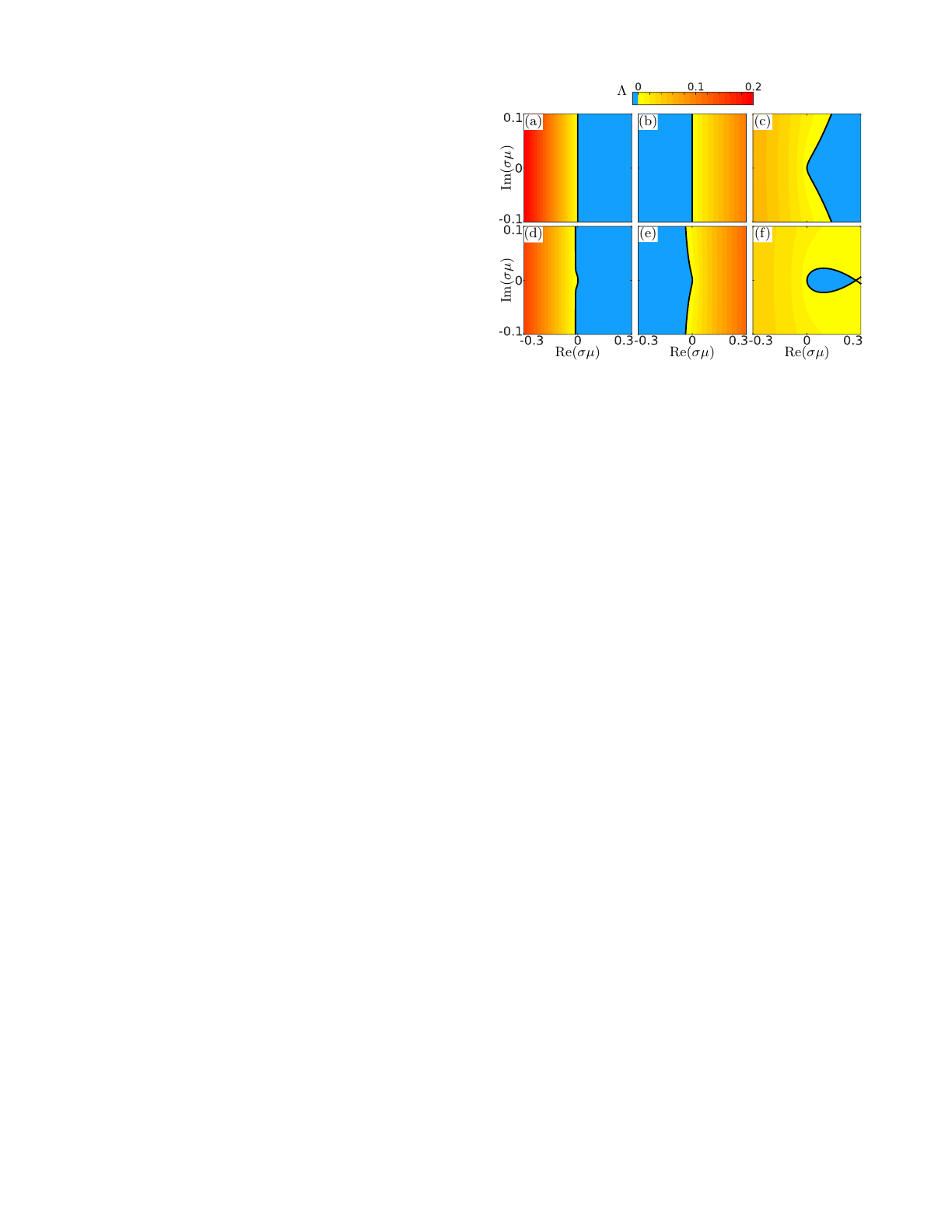
Figure 1 displays the master stability function deter-

mined for different adaptation rules controlled by β. The

blue-colored areas correspond to regions that lead to sta-

ble dynamics. By changing the control parameter β, var-

ious shapes of the stable regions are visible. For some

parameters, e.g., Fig. 1(c,d,e), almost a whole half-space

either left or right of the imaginary axis belongs to the

stable regime. This resembles the case of no adapta-

tion where the stability of the synchronous state is solely

described by the sign of the real part of σµ sin βcos α,

see Fig. 1(a,b). Note that in the case of no adaptation

(= 0) there exist N2neutral directions with zero eigen-

values that do not affect the stability, and correspond to

the variations of the coupling weights. We also find pa-

rameters where most values σµ correspond to unstable

dynamics, except for an island, i.e., a bounded region in

σµ parameter space, see Fig. 1(f).

To understand the emergence of the stability islands,

we analyze the boundary that separates the stable (Λ <

0) from the unstable region (Λ >0). This boundary is

given by the condition Λ = Reλ= 0, or, equivalently,

λ= iγ. Substituting this into Eq. (11), we obtain a pa-

rameterized expression for the boundary as a function

of γthat has the form σµ =Z(γ) with Z(γ) given ex-

plicitly in the Supplemental material [106]. The latter

(d) (e)

(a) (b)

Im(σµ) Im(σµ)

Re(σµ) Re(σµ)

(c)

(f)

Re(σµ)

FIG. 1. Master stability function Λ(σµ) for the adaptive

phase oscillator network (9)–(10). Regions belonging to neg-

ative Lyapunov exponents Λ are colored blue. The curve

where Λ(µ) = 0 is given as a black solid line. In panels (a)

and (b) the case without adaptation (= 0) is presented

for β=−0.35πand β= 0.2π, respectively. Other panels:

= 0.01 and (c) β=−0.95π, (d) β=−0.35π, (e) β= 0.2π,

and (f) β= 0.98π. In all panels α= 0.3π.

parametrization of the boundary is displayed in Fig. 1 as

the solid black line. It is straightforward to show that a

stability island exists if sin(α+β)/(cos αsin β)<0. The

latter condition indicates a certain balance between the

coupling and adaptation function. We emphasize that

the emergence of stability islands is a direct consequence

of adaptation. Without adaptation, the boundary sim-

plifies to the axis Re µ= 0, see Figs. 1(a,b). Intuitively,

the presence of adaptivity, i.e., Eq. (8), provides a feed-

back mechanism that can change the stability (e.g., by

an additional effective phase lag), and hence gives rise to

the emergence of stability islands of the master stability

function.

In the following, we analyze the behavior of the adap-

tive network of phase oscillators (9)–(10) in the presence

of a stability island, and show how such an island in-

troduces a desynchronization transition with increasing

overall coupling σ. To measure the coherence, we use the

cluster parameter RC[76, 79], which is given by the num-

ber of pairwise coherent oscillators normalized by the to-

tal number of pairs N2. In the case of complete synchro-

nization, frequency clustering, or incoherence, the cluster

parameter values are RC= 1, 1 < RC<0, or RC= 0,

respectively, see Supplemental Material for details [106].

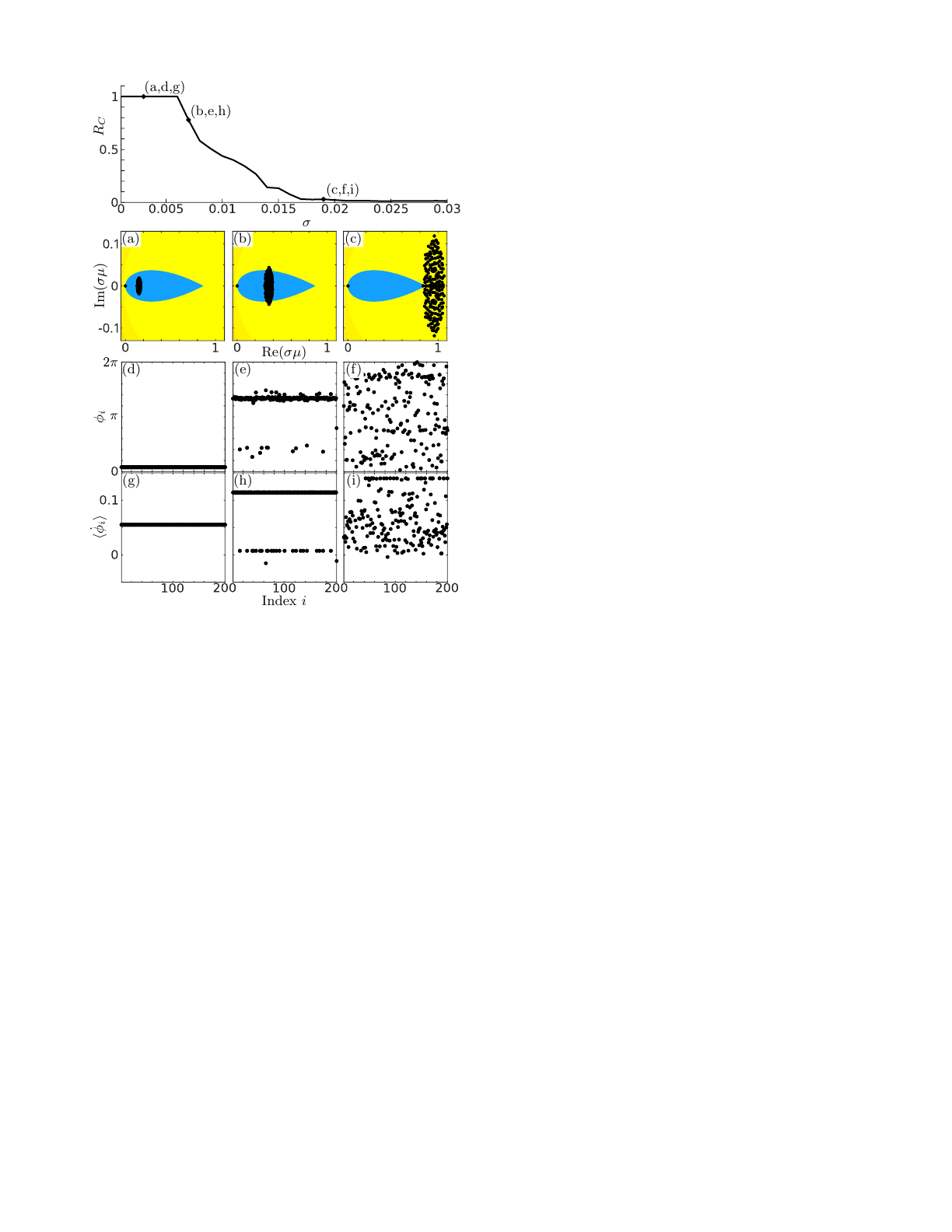
The top panel in Fig. 2 shows the cluster parameter

RCfor different values of the overall coupling constant

σ. We observe that for small σ, the synchronous state

is stable, see Fig. 2(a,d,g). This stability follows directly

from the master stability function since all values σµifor

all Laplacian eigenvalues lie within the stability island,

see Fig. 2(a).

(g) (h) (i)

Index i

(d) (e) (f)

Re(σµ)

(b)(a) (c)

(a,d,g)

(b,e,h)

(c,f,i)

φi

h˙

φiiRC

Im(σµ)

FIG. 2. Dynamics in the network of 200 oscillators (9)–(10)

with random adjacency matrix Ac[106], and different val-

ues of overall coupling strength σ. Adiabatic continuation for

increasing σwith the stepsize of 0.001, starting with the syn-

chronous state φi= 0, κij =−aij sin β. The top panel shows

the cluster parameter RCvs σ. For the three values of σ:

(a,d,g) σ= 0.003, (b,e,h) σ= 0.007, and (c,f,i) σ= 0.019,

the plots show: in (a,b,c) the master stability function color

coded as in Fig. 1, together with σµi, where µiare the N

Laplacian eigenvalues of Ac; in (d,e,f) snapshots for φiat

t= 30000; and in (g,h,i) the temporal average of the phase

velocities h˙

φiiover the last 5000 time units. Other parame-

ters: α= 0.49π,β= 0.88π,= 0.01.

By increasing the coupling strength σ, the values σµi

move out of the stability island (µiremain the same), and

the synchronous state becomes unstable, see Fig. 2(b,c).

For intermediate values of σ, multiclusters with hierar-

chical structure in the cluster size emerge, see Fig. 2(e,h)

for a three-cluster state. Increasing the coupling con-

stant further leads to the emergence of incoherence. In

Fig. 2(f,i), the coexistence of a coherent and an inco-

herent cluster is presented. Such chimera-like states

have been numerically studied for adaptive networks in

[76, 78, 79].

In the following, we show how our findings are trans-

ferred to a more realistic set-up of coupled neurons with

synaptic plasticity. For this, we consider a network

of FitzHugh-Nagumo neurons [93–96] coupled through

chemical excitatory synapses [97–99] equipped with plas-

ticity. The form of the synaptic plasticity is similar to

the rules used in [84, 100], with control parameters β1

and β2of the adaptation function which are uniquely

determined by the values of h(0) and Dh(0) of the plas-

ticity rule, and these are the only essential parameters

of the plasticity function, regarding the stability of the

synchronous state, see Eqs. (7)–(8). For more details on

the model, we refer to [99, 106].

The synchronous state of the network of FitzHugh-

Nagumo neurons satisfies Eqs. (3)–(4), and it is periodic

for the chosen parameter values. Using our extended

master stability approach, we determine numerically the

master stability function which is the maximum Lya-

punov exponent of Eqs. (7)–(8).

In Fig. 3(a,b,c), we show the master stability function

in dependence on the parameter µ/r for different values

of the overall coupling constant σ. We observe a sta-

bility island for the chosen set of parameters, see the

Supplemental material for other parameter values [106].

In contrast to the phase oscillator network in Fig. 2, the

shape of the master stability function does not scale lin-

early with σ. This is due to the non-diffusive coupling

function, see [106] for details. Moreover, with increasing

σ, the size of the stability island shrinks. Since all Lapla-

cian eigenvalues µiare independent of σ, we observe that

µi/r move out of the stability island with increasing σ.

For the globally coupled network, in particular, we have

either µi/r = 0 or µi/r = 1. Therefore, with increas-

ing σ, we find a transition from complete coherence, see

Fig. 3(a,d,g) to partial synchronization and incoherence.

We further observe that closely after destabilization, a

large frequency cluster remains visible, see Fig. 3(b,e,h).

For higher overall coupling, the cluster sizes shrink, and

the number of small clusters increases, see Fig. 3(c,f,i).

In summary, we have developed a master stability ap-

proach for a general class of adaptive networks. This

approach allows for studying the subtle interplay be-

tween nodal dynamics, adaptivity, and a complex net-

work structure. The master stability approach has been

first applied to a paradigmatic model of adaptively cou-

pled phase oscillators. We have presented several typ-

ical forms of the master stability function for different

adaptation rules, and observed adaptivity-induced sta-

bility islands. Besides, we have shown that stability is-

lands give rise to the emergence of multicluster states and

chimera-like states in the desynchronization transition

for an increasing overall coupling strength. Qualitatively

the same phenomena have been shown for a more realis-

tic network of non-diffusively coupled FitzHugh-Nagumo

neurons with synaptic plasticity. In this set-up, the emer-

gence of a stability island and a desynchronization tran-

sition have been found as well.

The theoretical approach introduced in this Letter pro-

Loading more pages...