Observations on the Relationship between Crash Frequency and Traffic Flow [original]

safety

Article

Observations on the Relationship between Crash Frequency

and Traffic Flow

Peter Wagner 1,2,* , Ragna Hoffmann 1and Andreas Leich 1,*





Citation: Wagner, P.; Hoffmann, R.;

Leich, A. Observations on the

Relationship between Crash

Frequency and Traffic Flow. Safety

2021,7, 3. https://doi.org/10.3390/

safety7010003

Received: 25 October 2020

Accepted: 7 January 2021

Published: 11 January 2021

Publisher’s Note: MDPI stays neu-

tral with regard to jurisdictional clai-

ms in published maps and institutio-

nal affiliations.

censee MDPI, Basel, Switzerland.

This article is an open access article

distributed under the terms and con-

ditions of the Creative Commons At-

tribution (CC BY) license (https://

creativecommons.org/licenses/by/

4.0/).

1Deutsches Zentrum für Luft- und Raumfahrt e.V., Institute of Transportation Systems, Rutherfordstrasse 2,

D-12489 Berlin, Germany; ragna.hoffmann@dlr.de

2Institute of Land- and Sea Transport Systems, Technical University of Berlin, Salzufer 17-19,

D-10587 Berlin, Germany

*Correspondence: peter.wagner@dlr.de (P.W.); Andreas.Leich@dlr.de (A.L.); Tel.: +49-30-67055-237 (P.W.)

Abstract:

This work analyzes the relationship between crash frequency

(crashes per hour) and

exposure

(cars per hour) on the macroscopic level of a whole city. As exposure, the traffic flow

is used here. Therefore, it analyzes a large crash database of the city of Berlin, Germany, together

with a novel traffic flow database. Both data display a strong weekly pattern, and, if taken together,

show that the relationship

N(Q)

is not a linear one. When

is small,

grows like a second-

order polynomial, while at large

there is a tendency towards saturation, leading to an S-shaped

relationship. Although visible in all data from all crashes, the data for the severe crashes display a

less prominent saturation. As a by-product, the analysis performed here also demonstrates that the

crash frequencies follow a negative binomial distribution, where both parameters of the distribution

depend on the hour of the week, and, presumably, on the traffic state in this hour. The work presented

in this paper aims at giving the reader a better understanding on how crash rates depend on exposure.

Keywords: road safety; traffic states; crash rates; temporal crash rate pattern

1. Motivation

Recent years have seen some progress when it comes to the availability and analysis of

crash data [

–

], or [

]. This has triggered new work and new methods, most notably from

machine learning that have the potential to improve knowledge, models, and, ultimately,

also the state of traffic safety.

In many cases, road safety work consists of identifying crash blackspots, determining

corrective measures, implementing them, and later evaluating them. A reasonable defini-

tion of a road accident blackspot will involve the number of crashes per unit of exposure.

This paper deals with the problem of modeling the relationship between crash rates and

exposure. A better understanding of this relationship allows traffic safety management

targeting hazardous locations more clearly based on risk and not merely on crash frequency.

Traditionally, one approach in this context is the development of crash prediction

models. They estimate the impact of several variables

xj·

on crash frequencies. This is done

by applying models of the type [5–9]:

Ni=β0(Qi/Q0)β1exp(µi) = β0(Qi/Q0)β1exp n

∑

j=2

βjxji +ζ!, (1)

where

is the crash frequency at a certain instance

(time, place,...),

is an exposure

variable,

is a baseline flow,

µi

is the mean value of the crash rate, the

xij

are factors

thought to influence the crash frequency, and the

βj

are coefficients that quantify the

strength of each factor. Moreover, there is a gamma-distributed noise term

here where

exp(ζ)has mean one and variance γ.

The crash frequencies themselves are then found as a realization of a stochastic process

with a negative binomial distribution (NBD) with a mean µand variance σ2:

Safety 2021,7, 3. https://doi.org/10.3390/safety7010003 https://www.mdpi.com/journal/safety

Safety 2021,7, 3 2 of 18

σ2=µ+γµ2. (2)

The parameter

describes how much the NBD deviates from a Poisson distribution,

with γ=0 for a Poisson distribution.

The exposure variable, which in the following will be mainly the traffic flow, is difficult

to include properly in traffic safety analyses. This is due to the fact that crashes are rare

events, and that more often than not, a measurement of the exposure is not available at

the site and time of the crash. If available, it is often only in the form of an average over

a day, and very often from travel demand models instead of directly measured. Similar

difficulties plague the other data source of exposure, which is the one that stems from

travel surveys. In many cases, they are averages over large spatial areas (as in travel survey

data) although attempts exist to integrate traffic flow with more detail [

–

]. However, it

might be speculated that crash probabilities depend strongly on the traffic state itself, with

traffic flow being one of the major influencing variable [14,15].

Especially of interest is the relationship between the crash frequency

when dis-

played versus the traffic flow

, see [

]. Note that often not

itself is displayed as a

function of Q, the crash rate ρis used instead:

ρ(Q) = N(Q)

Q. (3)

The crash rate is the ratio between an average crash frequency and the corresponding

average traffic flow, leading to a continuous variable. As is demonstrated in

Section 3.1

another interpretation is to use the discrete number of crashes in one hour and the associ-

ated traffic flow in this hour, which leads to a mixture between a discrete and a continuous

distribution. (A similar approach can be found in [

], they have used the mileage on the

x-axis.)

Some thoughts about the relationship between

N(Q)

and

ρ(Q)

are in order. It is very

likely that the crash rate does not vanish as a function of

, even for very small exposure

we expect that the crash rate does not drop to zero, and the results of this work will lend

additional credibility to this idea. So:

N(Q)∝Q⇔ρ(Q)∝ρ0for Q→0. (4)

For freeway traffic, a good deal of results for

N(Q)

and

ρ(Q)

are available. The most

commonly used model has a roughly U-shaped form for

ρ(Q)

, where crash rates are rather

large for small and large flows and have a minimum for intermediate flows. e.g., the

work [17,18] claims:

ρ(Q) = c1Q−β1+c2Qβ

2. (5)

where the exponent

β1

is around 1, and

β2

is between 1 and 2. Note that it is assumed that

the flow values are normalized to a constant flow so that the units drop out. The first term

is for single-vehicle crashes, while the second term describes multi-car crashes. Ceder also

observed that one should discern free traffic from congested traffic; this, however, raises

the question of how to do this properly based on hourly values. Furthermore, a recent

meta-analysis [

] that used 118 studies come to a similar conclusion, albeit with different

exponents β1,β2.

Similar results exist [

] or the German study [

], sometimes more symmetric

second-order polynomial relationships

ρ(Q)∝c1(Q−Qc)2+c0

have been used to describe

the data. The approach of [

] is a bit different since it displays crash rate as a function of

a novel indicator that is difficult to translate into traffic flow or volume/capacity ratios.

Note as an oddity that one of the earliest models on this topic [

] proposed an inverse

U-shaped relationship, which is once again a second-order polynomial; this time, the crash

rate is being small for small flow and large flows, which were in this case AADT values

(AADT = annual average daily traffic). However, Veh’s data are also consistent with the

assumption that the crash rate is constant, or a weakly increasing function of exposition.

Safety 2021,7, 3 3 of 18

In essence, it could be stated that currently there is no univocal picture about the

relationship

ρ(Q)

for freeway data; for a more complete overview see [

]. Note, however,

that at least the idea of a diverging crash rate for

Q→

0 might be questionable; however,

this is not the topic of this work.

Results are different when looking at the relationship between

and AADT as an

exposure variable. In this case, crash rates increase with

, eventually again as a power-law

ρ(Q)∝Qβ[26].

Very little work has been done so far that looks at the relationship

N(Q)

on the basis

for a whole city, with notable exceptions of [

] with a more theoretical approach, and [

]

trying to test this theory without having real flow data available, and the recent work on a

network-based macroscopic safety diagram [29].

The hypothesis behind this work was the assumption that at least the crash frequency

that involves two cars should be a second-order polynomial function of the traffic flow [

A similar idea is also proposed in [

]. Therefore, a reasonable model for the crash

frequency in a city is a combination of single-car crashes (which can be assumed to be

proportional to the number of vehicles around

) and an interaction term proportional to

. This interaction term is due to a naive assumption that if vehicles move independently

of each other, then there is a probability proportional to Q2that they meet:

N=α1Q+α2Q2(6)

Note that it is not easy to bring Equation (6) in line with Equation (1): the latter

one is tailored towards the use of generalized linear models (GLM) with a logarithmic

link function, and by exchanging

Qβ1

with

α1Q+α2Q2

, the very character of this model

is changed into something that no longer can be treated as GLM with a logarithmic

link function.

However, this work deals only with the prefactor and ignores

exp(µi)

, so a GLM and

its generalization GAM (generalized additive model) can still be used, but in most cases

with the identity as the link function.

As a final remark, note that models with a power-law term as in Equation (1) are not

in line with the assumption in Equation (4) that the crash rate becomes constant for small

exposure. However, when looking closely into [

], then Equation (5) function might be

modified to avoid the divergence at

Q→

0 by modifying the first term in the equation into

c1(Q+b)−β1.

2. The Data

This paper uses two types of data. The first one is a large crash database that contains

all crashes reported by the Berlin police in the city of Berlin, Germany, during the years

2001–2019

. The data are de-identified, i.e., they do not contain numberplates or names

of the crash participants or any other information that can be used to identify them.

Furthermore, for the subset of data used in the work reported here, the crash-time has been

aggregated to the hour.

Note that common practice in Berlin is different from other German federal states since

even a lot of property damage only (PDO) crashes are reported in the database. However,

even here the analyst must be aware of the fact that these numbers are biased due to the

under-reporting of small crashes. For this paper, only some part of the data in this database

has been used, see below for a more detailed description.

The second set of data stems from the Traffic4cast competition [

]. It contains de-

identified data from most of the days of 2018 in Berlin, where the speeds and the number of

probes of a certain vehicle fleet have been recorded. Since such a data set is a bit unusual, it

has been complemented by two other de-identified data sets so that comparisons between

the different data could be performed that are interesting in their own right. These are

the annual hourly count data from 28 detection sites, which have been provided by the

German Federal Highway Research Institute (BASt) and data from the latest travel survey

in Germany named Mobility in Deutschland (MiD) [33].

Safety 2021,7, 3 4 of 18

2.1. The Crash Database

The crash database has been provided by the Berlin police, and it is not publicly

available. It contains for each crash

about 60

×ni

variables (some redundant), where

the number of people involved in the crash. Here, only the time

, the severity, and the

vehicle types have been used. Time is described with minutes’ resolution; however, it is

good not to use these numbers to this precision since preference for multiples of 15 min can

be observed (see also [

]). The severity of each crash is described by the number of lightly

injured, the number of severely injured, the number of fatalities, and the damage.

In the following, only severe (crashes with injured or killed participants) and non-

severe PDO crashes will be distinguished. The database contains 1,888,038 crashes, and

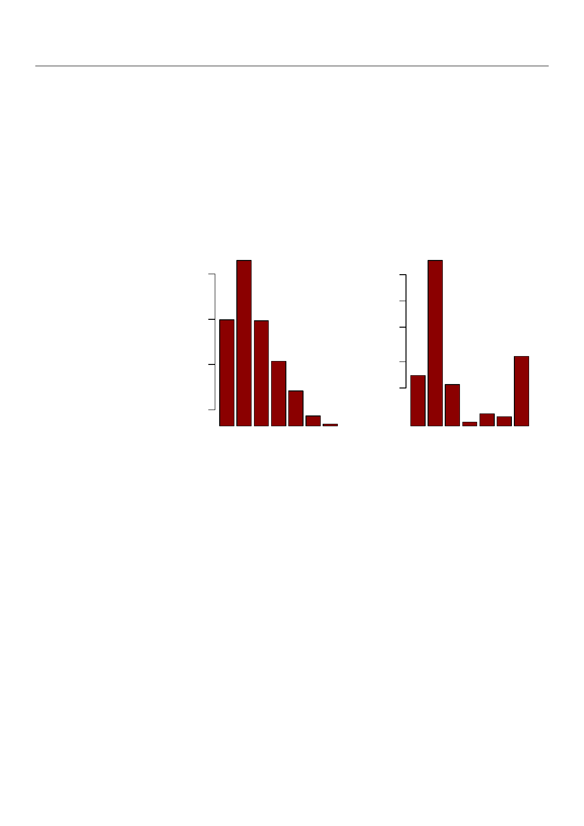
what is important for the analysis below: most of all crashes are between two cars, as can

be seen in Figure 1.

123456

# crash participants

Counts

10k

100k

4.42%

4.17%

0.53%

0.12%

0.03%

0.02%

90.7%

Bike

Car

Misc

MoBike

Peds

PT−Bus

Truck

Counts

3.93%

82.59%

3.09%

6.5%

1.14%

1.43%

1.32%

100k

200k

500k

Figure 1.

Distribution of the number of road users involved (

left

), and the traffic shares (

right

) in the

Berlin crash data set. The Misc traffic mode is being used by the police to denote any traffic mode

that cannot be assigned. The

-axis is logarithmic, the numbers on top of the bars are the percentages

of the respective shares.

For this study, the timestamps of all crashes of the database have been rounded down

to the nearest full hour and translated to the corresponding hour of the week (0–167). Since

the data set spans 19 years, each hour occurs 992 times in the data set, resulting in 992

crash numbers for every hour of the week

. Therefore, for each hour of the week, the

distribution of counts can be determined directly. The results are displayed in Figure 2as a

boxplot, and they display a strong weekly pattern. Very similar results have been reported

recently by [34].

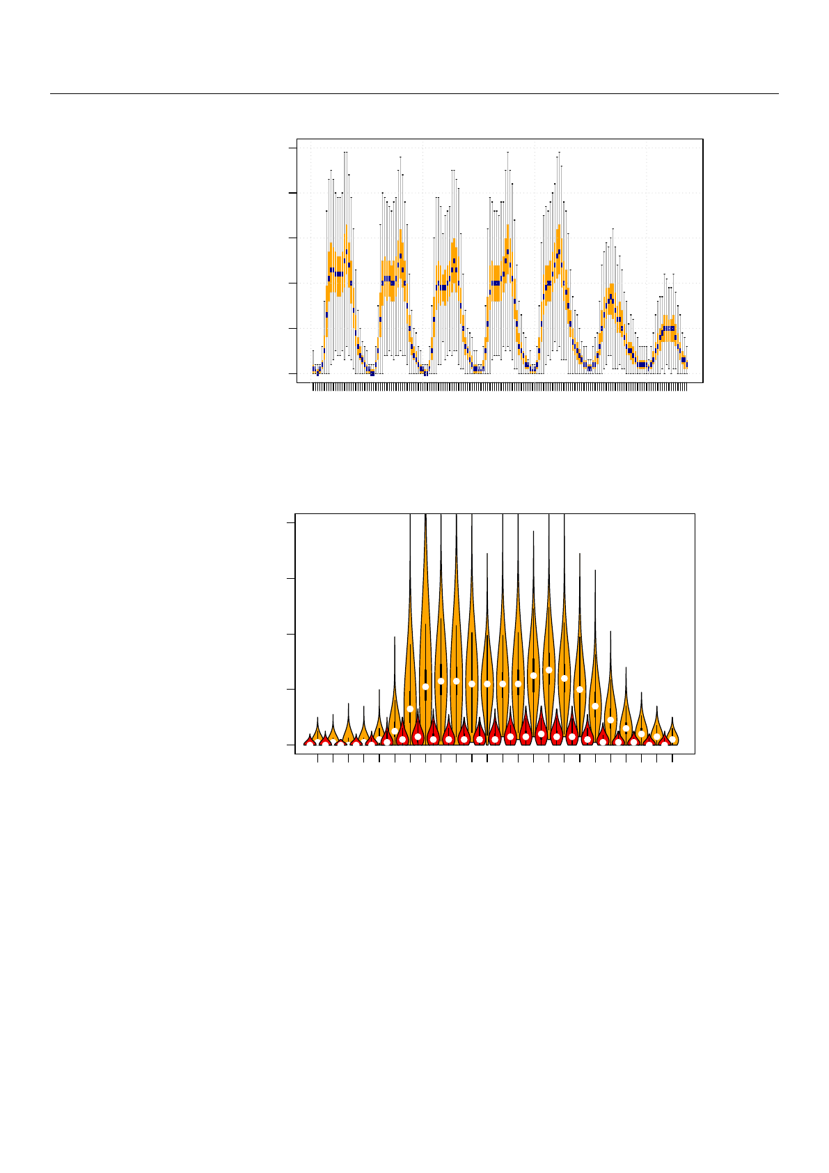
The Figure 3displays this result for the Monday only as a violin plot so that the shape

of the distributions can be seen more clearly. Moreover, the distribution of severe crashes

has been included in this Figure as well.

Safety 2021,7, 3 5 of 18

0 9 20 32 44 56 68 80 92 106 122 138 154

Hour of week h

N(h) (Counts/h)

Figure 2.

Box plot of the crash frequency per hour of the week. The blue bar is the median, the boxes

are the 25- and 75-percentiles, the whiskers display the minimum and the maximum of the data.

0 2 4 6 8 10 12 14 16 18 20 22

Hour of Monday (h)

N(h) (Counts/h)

Figure 3.

Distribution of the hourly crash counts as a function of the hour of the day on Mondays,

displayed as a violin plot. The orange violins are for all crashes, the red ones for the severe crashes

(which are shifted left by half an hour). The white circle is the median of the values.

2.2. The Distribution of the Crash Frequency

Most likely, the individual distributions in each hour are following an NBD. This can

be tested by plotting their variance

σ2

against their mean value

. An NBD displays then a

second-order polynomial relationship between µand σ2as stated already in Equation (2),

where the parameter

specifies the deviation of the distribution from a Poisson distribution.

The results can be seen in Figure 4. Figure 4shows that the data follow an NBD. Also, the

same analysis has been performed for severe crashes only. Various fits to this cloud of data-

points have been included in this Figure as well demonstrating that the assumption of the

NBD fits these data quite well. All fits are done with R’s

lm()

function [

], which executes

a linear least-squares fit to these data. The fit for the severe crashes is even better (larger

leading to two different estimates for the

variable. For all crashes,

is estimated as

Loading more pages...