
SoftwareX 16 (2021) 100871
Contents lists available at ScienceDirect
SoftwareX
journal homepage: www.elsevier.com/locate/softx
Original software publication
AnyMOD.jl: A Julia package for creating energy system models
Leonard Göke
TU Berlin, Workgroup for Infrastructure Policy (WIP), Straße des 17. Juni 135, 10623 Berlin, Germany
article info
Article history:
Received 2 November 2020
Received in revised form 9 September 2021
Accepted 19 October 2021
Keywords:
Macro-energy systems
Energy system modeling
Open-source modeling
Julia
abstract
AnyMOD.jl is a Julia framework for creating large-scale energy system models with multiple periods
of capacity expansion. It applies a novel graph-based approach that was developed to address the
challenges in modeling high levels of intermittent generation and sectoral integration. Created models
are formulated as linear optimization problems using JuMP.jl as a backend.
To enable modelers to work more efficiently, the framework provides additional features that help
to visualize results, streamline the read-in of input data, and rescale optimization problems to increase
solver performance.
©2021 The Author. Published by Elsevier B.V. This is an open access article under the CC BY license
(http://creativecommons.org/licenses/by/4.0/).
Code metadata
Current code version v0.1.6
Permanent link to code/repository used for this code version https://github.com/ElsevierSoftwareX/SOFTX_2020_103
Code Ocean compute capsule
Legal Code License MIT license (MIT)
Code versioning system used git
Software code languages, tools, and services used Julia
Compilation requirements, operating environments & dependencies Julia 1.3.1
If available Link to developer documentation/manual https://leonardgoeke.github.io/AnyMOD.jl/stable/
Software metadata
Current software version v0.1.6
Permanent link to executables of this version https://github.com/leonardgoeke/AnyMOD.jl/releases/tag/v0.1.6
Legal Software License MIT license (MIT)
Computing platforms/Operating Systems Linux, Microsoft Windows, iOS
Installation requirements & dependencies Julia 1.3.1
If available, link to user manual - if formally published include a reference to
the publication in the reference list
https://leonardgoeke.github.io/AnyMOD.jl/stable/
1. Motivation and significance
Since the production of energy accounts for three-quarters of
global emissions, mitigating climate change requires the decar-
bonization of the energy system [1]. Cutting emissions requires to
shift supply of primary energy to electricity from wind and solar
and extend its use to other sectors. As a result, the energy system
has to undergo fundamental change and evolve from largely
independent sectors with little supply from renewables into an
integrated system characterized by fluctuating renewables.
Capacity expansion models investigate the long-term develop-
ments of macro-energy systems, but existing methods were de-
veloped for systems still characterized by fossil fuels and struggle
to describe the transformation towards a renewable system [2].
Models like ReEDS, Message, or Switch, pursue a time-slice ap-
proach, that reduces the entire year to a small number of inde-
pendent periods [3–5]. This reduction limits the detail applied to
fluctuating renewables and more importantly prohibits to con-
sider long-term storage, a key component of renewable energy
https://doi.org/10.1016/j.softx.2021.100871
2352-7110/©2021 The Author. Published by Elsevier B.V. This is an open access article under the CC BY license (http://creativecommons.org/licenses/by/4.0/).

Leonard Göke SoftwareX 16 (2021) 100871
systems [6,7]. Other models, like PyPSA or Calliope, diverge from
this approach and consider a continuous and hourly time-series
instead, which enables a detailed representation of renewables
and long-term storage [8,9]. But in return these models are lim-
ited to a single year and, opposed to models using time-slices,
cannot analyze development pathways for today’s system.
Against this background, AnyMOD.jl provides a framework
for modeling the long-term transformation of the energy system
with the level of detail necessary to represent fluctuating renew-
ables and long-term storage. The framework implements a novel
graph-based method introduced in Göke [10] that varies the level
of temporal and spatial detail by energy carrier to keep models
with high resolution computationally tractable. The approach also
enables to model the substitution of energy carriers and, on the
practical side, facilitates the read-in of input data.
AnyMOD.jl follows an easy to use, but difficult to master
principle. Since individual models are solely defined by CSV files
and can be run with a few lines of standard code, running an
existing model, and performing sensitivity analysis requires little
experience. More advanced applications, like creating new mod-
els and individually modifying their formulation, requires some
programming skills and a deeper understanding of the frame-
work’s structure. Since models are defined from CSV files and
short code scripts, the framework supports version-controlled
model development to promote collaboration and transparency.
The following section gives an overview of the framework’s
structure and presents two functionalities with greater detail,
the read-in of parameter data (Section 2.2.1) and the re-scaling
algorithm (Section 2.2.2). The subsequent section describes an ap-
plication that models the transformation of the European power
and gas sector. The final section paper highlights the framework’s
impact and concludes.
2. Software description
The package is implemented in Julia. Its key dependencies are
JuMP.jl as a backend for linear optimization and DataFrames.jl for
data processing [11,12]. The framework uses PyCall.jl to create
an internal Python environment and apply the Python packages
NetworkX and Plotly for plotting. Gurobi is added as an optional
dependency, because its function to compute irreducible incon-
sistent subsystems is utilized to debug infeasible models. Apart
from that, the framework is compatible with any open or com-
mercial solver capable of interoperating with the JuMP.jl pack-
age.1To increase performance the package heavily utilizes Ju-
lia’s multi-threading capabilities. Since not supported by JuMP.jl,
the mere creation of constraints uses only one thread, but the
computationally more intensive composition of constraints from
variables and parameters is multi-threaded.
2.1. Software architecture
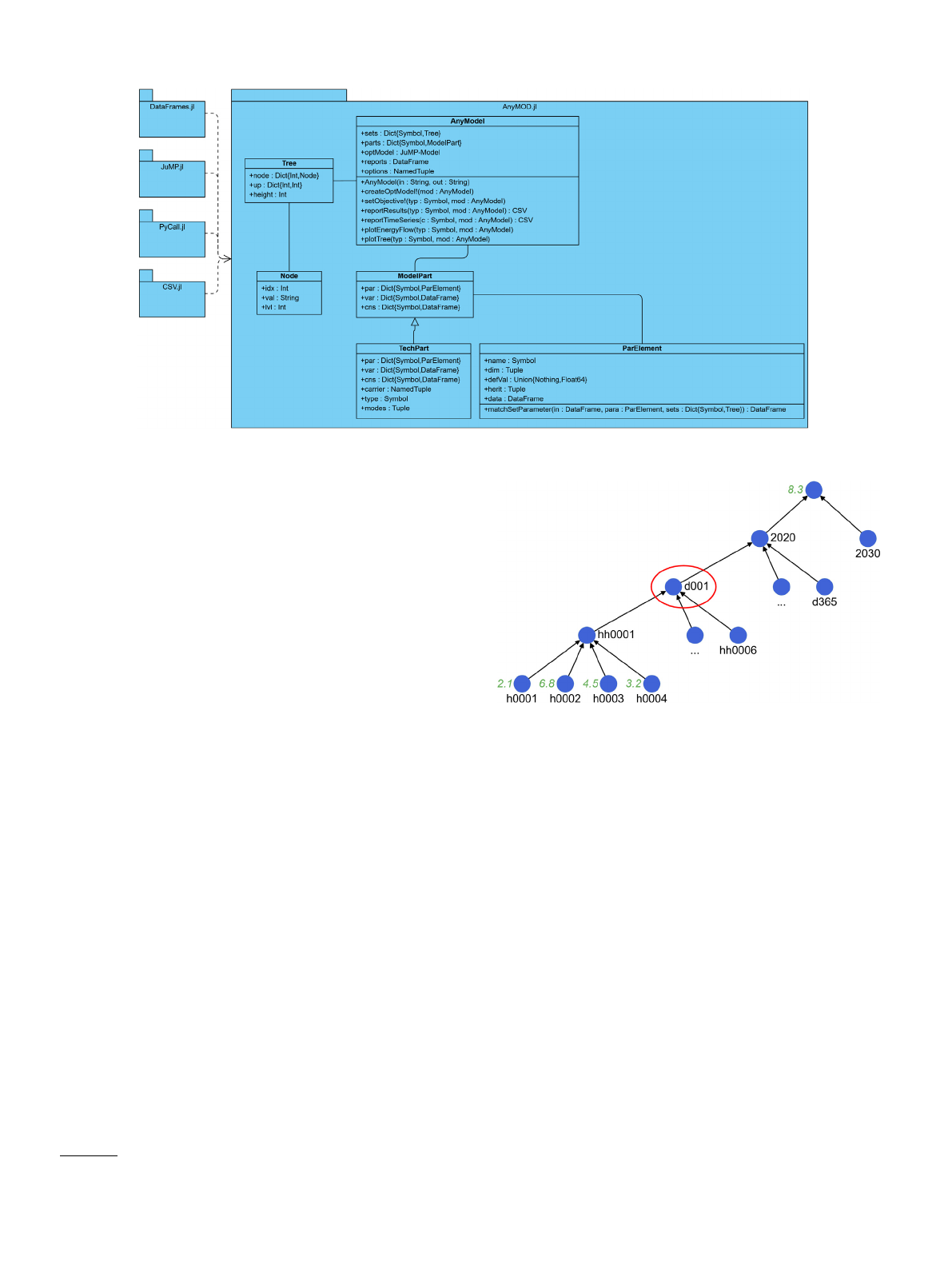
The class diagram in Fig. 1 illustrates the architecture of Any-
MOD.jl and how it revolves around the AnyModel object. For the
sake of clarity, the diagram is not exhaustive and only covers
the most relevant dependencies, objects and attributes. Listing 1
provides the corresponding code to initialize, populate, solve and
analyze the model object.
After loading AnyMOD.jl, the constructor initializes the
AnyModel object based on two mandatory arguments: an input
directory and an output directory. The CSV files defining a model
consist of set and parameter files that have to be placed in the
input directory. The set files define all time-steps, regions, energy
carriers and technologies considered in a model and map how
1JuMP.jl uses the package MathOptInterface.jl to interface solvers.
Table 1
Exemplary data frame of generation variables.
Time-step Region Carrier Technology Variable
1 1 1 1 gen(1,1,1,1)
2 1 1 1 gen(2,1,1,1)
3 1 1 1 gen(3,1,1,1)
Table 2
Exemplary data frame of energy balance constraints.
Time-step Region Carrier Constraint
1 1 1 dem(1,1,1) =∑tgen(1,1,1,t)
2 1 1 dem(2,1,1) =∑tgen(2,1,1,t)
3 1 1 dem(3,1,1) =∑tgen(3,1,1,t)
these are related, for example which carriers a technology can
generate. Following the graph-based approach, the elements of
each set are organized as nodes of hierarchical trees.
⊵
using AnyMOD # loading packages
model_object = anyModel("../demo","results")# construct model object
# create optimization problem and set an objective
createOptModel!(model_object)
setObjective!(:costs, model_object)
# solve model and report results
using Cbc
set_optimizer(model_object.optModel, Cbc.Optimizer)
optimize!(model_object.optModel)
reportResults(:summary, model_object)
Listing 1: Script to initialize, create and run a model
Qualitative inputs on sets are complemented with quantitative
data from the parameter files, that for instance provide demand
time-series or technology properties like investment costs or
efficiency. While the naming and format of set files is strictly
defined, parameter data can be freely structured and distributed
across files. As a result, models can be composed modularly, since
different models can share the same input files. After reading in
all parameter data, the constructor creates a ParElement object
for each parameter with data and meta information and assigns
it to a ModelPart object. The ModelPart objects partition the model
into different parts, for instance, the ParElement for demand
time-series will be assigned to a model part dedicated to the
energy balance. Each technology got its own part object of the
subclass TechPart, that also stores technology specific attributes
like assigned carriers.
After construction, the AnyModel object is passed to the cre-
ateModel! function, which creates all the variables and constraints
of the underlying optimization problem optModel. These variables
and constraints are again assigned to model parts and stored as
data frames. For instance, Table 1 depicts a data frame of gener-
ation variables. The column on the right stores the JuMP variable
objects and the four other columns give the time-step, region,
carrier, and technology of each variable, which are provided as
indexes of the Node objects created during initialization. Such
data frames for variables are combined with parameter data using
database operations to construct constraints. For instance, gener-
ation variables are aggregated by technology and than joined with
the demand parameter to create the energy balance in Table 2.
After the optimization problem is created, its objective is set
with the setObjective function. At this point the user can also
freely modify and extend the automatically generated problem by
accessing the JuMP attributes of the AnyModel object and its parts.
Finally, the optimization problem optModel is passed to a solver
and analyzed afterwards. All results are written to the output
directory, which was passed to the constructor in the beginning.
A reporting file with error messages and warnings is written to
this directory as well.
2
Leonard Göke SoftwareX 16 (2021) 100871
Fig. 1. UML class diagram of package components.
2.2. Software functionalities
As outlined above, AnyMOD.jl is a package for the creation of
energy system models. Additional features are aimed either at
simplifying its application or enhancing the performance of cre-
ating and solving models. In the following, two of these features
are presented in greater detail.
2.2.1. Inheritance algorithm
According to the previous section, model constraints are con-
structed from variables and parameters, which are again defined
by input data. Usually, models use a single parameter value in
many constraints. For example, the efficiency of a newly build gas
power plant does typically not vary by time-step or region and
all constraints describing these plants will use the same value.
Consequently, it would be inefficient, if AnyMOD.jl required users
to provide efficiency data at a temporal and spatial resolution. On
the other hand, efficiencies of heat-pumps are highly dependant
on region and time-step, because they depend on ambient tem-
perature. So, not permitting efficiencies to depend on time-step
and region, would prevent to model these technologies accu-
rately. A similar problem occurs, if investment costs of emerging
technologies, like photovoltaic, are expected to decrease within
the model horizon, but costs for other technologies remain con-
stant. Here, providing all costs at a yearly resolution leads to
redundant inputs for most technologies, but if costs cannot be
varied by year at all, cost degression of photovoltaic cannot be
modeled. In conclusion a predefined resolution of input data
either results in an highly inefficient read-in of input data or
restricts modeling capabilities.
To resolve this problem, AnyMOD.jl does not predefine the
resolution of input data and instead automatically infers how
data should be used from the way it is specified. For example,
providing different efficiencies in dependence of time-step and
region will result in temporally and spatially resolved efficiencies
in the model, but if instead a parameter is provided without time-
steps or regions, the model uses a uniform value. This concept
is not limited to certain parameters or dimensions, but applies
comprehensively. The implementing algorithm builds on the idea
to ‘‘inherit’’ missing data for a specific node from its relatives in
the hierarchical tree.2
2This idea of ‘‘inheritance’’ is not be confused with inheritance in the context
of object orientated programming.
Fig. 2. Basic mechanism of inheritance within hierarchical trees.
Fig. 2 illustrates the basic mechanism of the algorithm based
on an exemplary hierarchical tree organizing time-steps. The first
level of the tree organizes different years with days, 4-hours steps
and hours following on the subsequent levels. Green numbers
indicate input data provided for a specific node. If input data is
not specified in dependence of the time-step, it is assigned to the
root of the tree. The algorithm can obtain missing data at the
circled node in three different ways: either move up the tree and
use ‘8.3’, move down the tree and sum the hourly values, or move
down the tree and average the hourly values. How the algorithm
deploys these three methods for each dimension depends on the
inheritance rules of the parameter. A detailed overview for each
parameter is provided in the parameter list of the documentation.
Finally, it can be outlined how these rules are deployed to
obtain parameter data. The described algorithm corresponds to
the matchSetParameter function of ParElement in Fig. 1 and takes
the following inputs: a data frame to be filled with parameter
data, a respective parameter object and the hierarchical trees.
First, the algorithm checks for direct matches between the input
data frame and the parameter data. Afterwards, it loops over
the inheritance rules to inherit new data for missing nodes as
described above. If new data is obtained, the algorithm checks
again for matches with the input data frame. The loops ends
when either all rows are matched with data, or all inheritance
rules have been applied. In the latter case, unassigned rows are
3
Leonard Göke SoftwareX 16 (2021) 100871
Fig. 3. Impact of scaling algorithm on solver run-time.
either dropped or assigned a default value, if one is defined for
the respective parameter.
2.2.2. Scaling
The formulation of an optimization problem can have a major
impact on solver performance. The barrier algorithm, the fastest
method for solving large linear problems, is particularly sensitive
to a model’s numerical properties, and poor formulations will
thus greatly increase computation time. For this reason, Any-
MOD.jl automatically applies a two-step scaling process when
creating optimization problems. The process aims to narrow the
range of coefficients and constants in a problem between 10−3
and 106, as recommended.3
As a demonstration of how this range is achieved, Eq. (1)
constitutes the constraints of an exemplary linear model. In the
first and second row, the coefficients for x1are currently outside
of the targeted interval. In addition, the maximum range of coeffi-
cients in the second row amounts to 1011 (= 102
10−9), which exceeds
the maximum range of the targeted interval of 109(= 106
10−3) and
means the equation cannot be multiplied with a constant factor
to shift coefficients into the desired interval.
10−8x1+103x2+x3≤b1
10−9x1+102x2+x3≤b2
x1+x2+x3≤b2
(1)
Therefore, in the first step the maximum range of coefficients
is decreased by substituting variables. In the example, x1is substi-
tuted with 103x′
1, which results in the system displayed in Eq. (2).
10−5x′
1+103x2+x3≤b1
10−6x′
1+102x2+x3≤b2
103x′
1+x2+x3≤b2
(2)
Since the first step decreased the maximum range, in the
second step coefficients can be shifted into the interval between
10−3and 106. For this purpose, each constraint (or row) is scaled
with a constant factor. In the example, the first row is multiplied
by 102and the second row by 103resulting in the system dis-
played in Eq. (3) that finally complies with the recommended
range.
10−3x′
1+105x2+102x3≤102b1
10−3x′
1+105x2+103x3≤103b2
103x′
1+x2+x3≤b2
(3)
AnyMOD.jl uses default factors for substitution that depend on
the variable type and can be adjusted if they fail to achieve the
desired result. Factors for scaling can be automatically computed
based on the current coefficients in a constraint.
3See the Gurobi Guidelines for Numerical Issues for details.
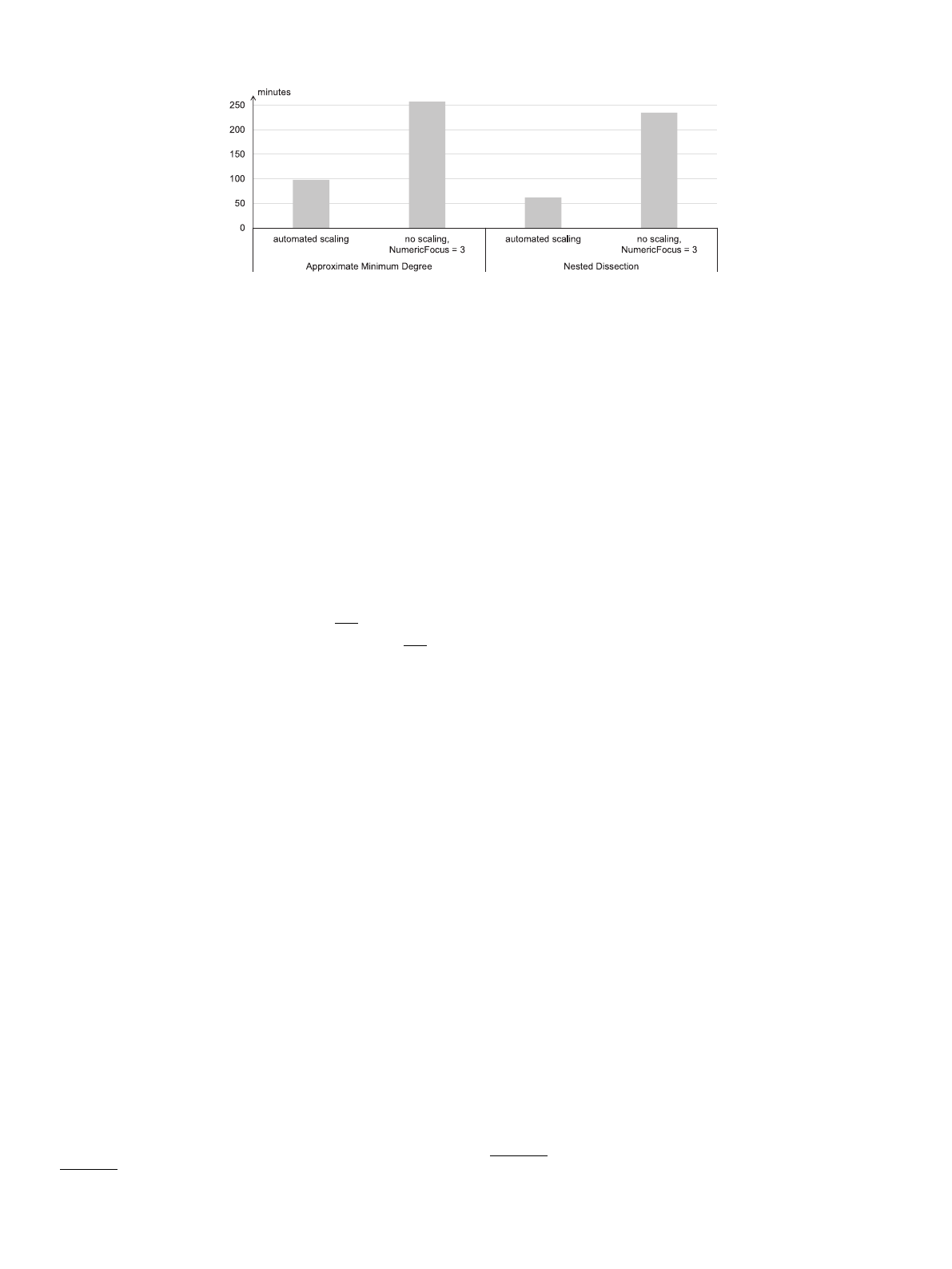
Fig. 3 demonstrates the impact of automated scaling by com-
paring the solve times of Gurobi’s barrier implementation for
a test model.4To ensure robustness of the results, Barrier was
run with both available ordering algorithms, ‘‘approximate min-
imum degree’’ and ‘‘nested dissection’’. With automated scaling
disabled, a NumericFocus parameter of three is necessary to avoid
early termination or extremely long solve times due to numerical
difficulties. In conclusion, automated scaling decreases solve time
of the test model roughly by a factor of three.
3. Illustrative example
Hainsch et al. [13] applied AnyMOD.jl to the decarbonization
of the European power and gas sector on a pathway from 2030
to 2040 instead of a single year. The analysis with AnyMOD.jl
complements results from another energy system model with
less spatiotemporal detail. The application subdivides Europe on a
country level and includes an aggregated representation of trans-
mission infrastructure to enable the exchange of energy carriers
between countries.
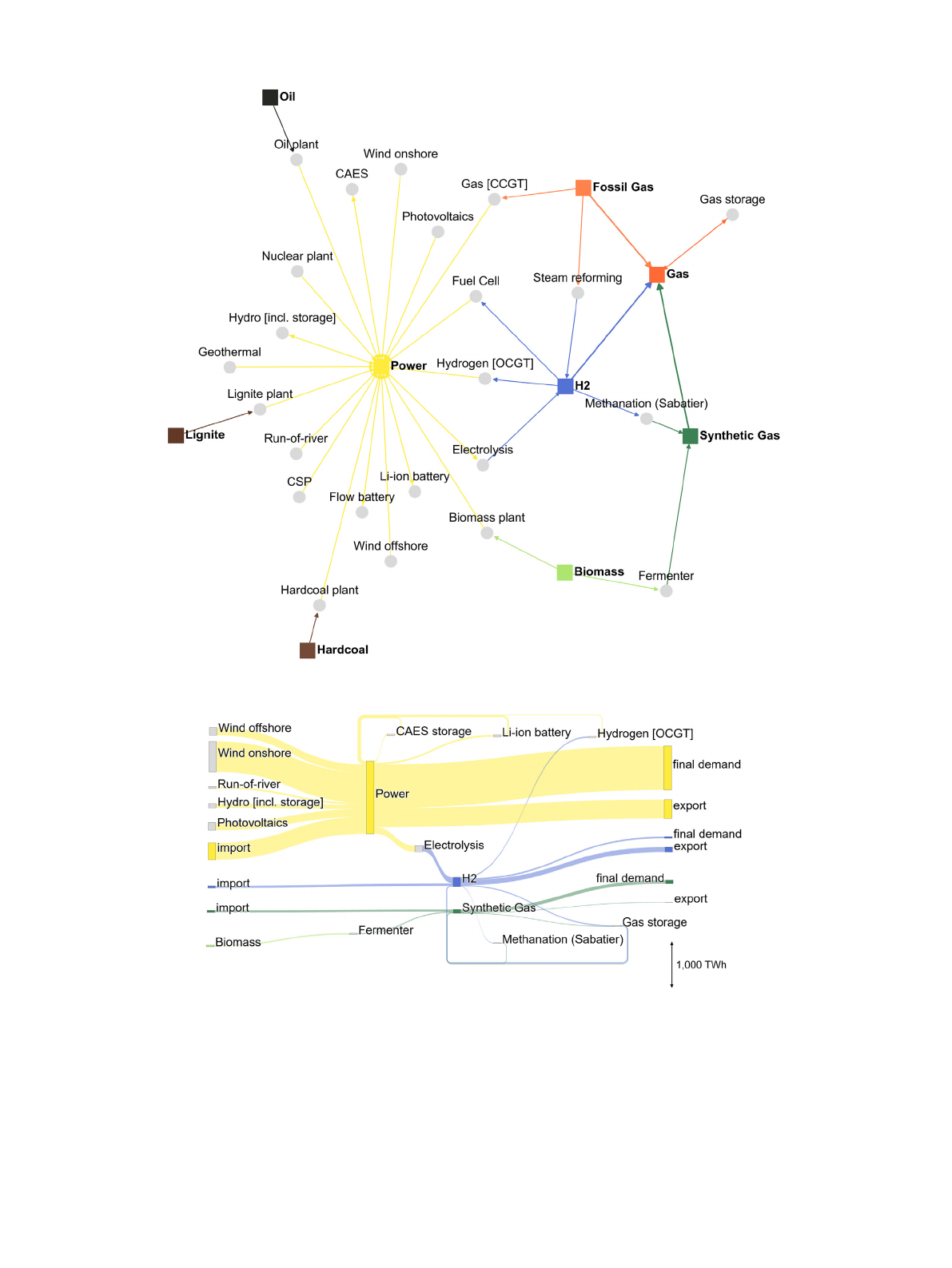
Fig. 4 was plotted with the plotEnergyFlow function and pro-
vides an overview of the technologies and energy carriers con-
sidered. In the graph, carriers are symbolized by colored vertices
and technologies by gray vertices. Entering edges of technologies
point towards their input carriers; outgoing edges refer to out-
puts. Since the model includes both the power and gas sector, it
is not limited to short-term storage of power, like batteries, but
also considers creation and utilization of synthetic fuels for long-
term storage. Since fluctuating renewables are the main source
of supply by 2040, power is modeled at an hourly resolution.
To reduce model size and account for the inherent flexibility of
gaseous energy carriers, fossil gas, hydrogen, and synthetic gas
are balanced daily instead. All other energy carriers are modeled
yearly.
The energy flows for France in 2040 when solving the model
are displayed in Fig. 5. The sankey diagram does not only show
how hydrogen is used for long-term storage of power, but also
how final demand for hydrogen and synthetic gases, for example
from the industry sector, is covered. In addition, the substantial
amount of imports and exports for all carriers highlights the
importance of large models that can account for several regions
at once.
4. Impact and conclusions
AnyMOD.jl provides a framework for modeling the transfor-
mation towards a decarbonized energy system at a high spa-
tiotemporal resolution. For this purpose, it implements a graph-
based method introduced that enables to vary the level of detail
4The corresponding model files can be found in the following repository:
https://github.com/leonardgoeke/AnyMOD_example_model/tree/May2020.
4
Leonard Göke SoftwareX 16 (2021) 100871
Fig. 4. Graph of technologies and energy in example.
Fig. 5. Sankey diagram for France in 2040 in example.
by energy carrier. In addition, the framework introduces a more
flexible method to read-in input data and automatically scales
created optimization problems to increase solver performance.
Lastly, the tool provides advanced plotting features, like Sankey
diagrams.
To facilitate access for users, AnyMOD.jl can be used without
any proprietary software. Using the framework does not require
extensive programming skills but supports version-controlled
model development, since models are created from CSV files.
To extend and modify a created model, advanced users can
easily access and manipulate its underlying JuMP objects. The
organization of input files is highly flexible and eases the creation
of new models from existing files.
In conclusion, AnyMOD.jl enables research to spend less time
on coding and data management and more time focusing on
the scientific part of their work. Its high level of accessibility
also makes AnyMOD.jl suitable for use by companies, regulators,
or non-governmental organizations. Finally, AnyMOD.jl promotes
5
Loading more pages...