Impact structures on Mercury from MESSENGER data: Implications on their formation processes and crustal structure [original]

Contents lists available at ScienceDirect

Icarus

journal homepage: www.elsevier.com/locate/icarus

Research Paper

Impact structures on Mercury from MESSENGER data: Implications on their

formation processes and crustal structure

Claudia Camila Szczecha,b,∗, Jürgen Oberst b, Alexander Starka, Hauke Hussmann a,

Frank Preusker a

aGerman Aerospace Center (DLR), Institute of Planetary Research, Berlin, Germany

bInstitute of Geodesy and Geoinformation Science, Technische Universität Berlin, Berlin, Germany

ARTICLE INFO

Keywords:

Mercury

Surface

Interior

Impact processes

Geophysics

ABSTRACT

In this study high-resolution stereo images and Digital Terrain Models (DTMs) from MErcury Surface, Space

ENvironment, Geochemistry and Ranging (MESSENGER) mission were utilized to detect impact structures in

regions not covered by Mercury’s Laser Altimeter (MLA), while gravitational data was utilized as a supported

data set. We have established an inventory of 314 impact structures ≥150 km, classified on their morphological

and gravitational characteristics. 24 basins ≥300 km have been newly discovered. Additionally, we have

identified significant surface modifications in impact structures of smooth material infill, which can be either

impact-induced or volcanic in origin. The Bouguer anomaly and crustal thinning in the center are displaying

an interplay of predominant change of crustal structure in impact basins. Further, this study reveals a common

impact history of Mercury and the Moon. Nevertheless, cumulative density distributions suggest the possibility

of either a divergence in impactor populations responsible for forming large basins on both celestial bodies

or a significant shift in impactor rates. This work holds important implications not only for understanding

impact structure formation and evolution processes but also for interpreting the crustal structure. It presents

an updated and expanded catalog of impact structures on Mercury, encompassing buried basins, and identifies

new areas of interest, potentially serving as target sites for the forthcoming BepiColombo mission.

1. Introduction

Impact structures are predominant surface features on Mercury

(Head et al.,2010;Baker et al.,2011;Fassett et al.,2012;Fassett,

2016), yet their formation and evolution processes are not fully un-

derstood (Head,2010;Fassett et al.,2017). This uncertainty partly

arises from the lack of understanding of surface and subsurface defor-

mation processes related to impact formation. Previous studies based

on MErcury Surface, Space ENvironment, Geochemistry and Rang-

ing (MESSENGER) mission data have cataloged and characterized 94

impact basins (≥300 km) (Fassett et al.,2017;Orgel et al.,2020).

However, because the identification of these impact structures was

based on image and topography data only, where recognition of details

depended on resolution and illumination conditions, this early catalog

is likely to suffer from biases.

Recent studies utilized gravity models of Mercury to gain insights

into Mercury’s subsurface structure (Genova et al.,2019;Konopliv

et al.,2020;Goossens et al.,2022). Those gravity models deliver

information that improves on understanding impact structures and

their related subsurface structures. Topography and gravity data with

∗Corresponding author at: Institute of Geodesy and Geoinformation Science, Technische Universität Berlin, Berlin, Germany.

E-mail address: [email protected] (C.C. Szczech).

good spatial resolution are limited to the high northern latitudes of

Mercury due to the eccentric orbit of the spacecraft. A complete search

and assessment of the basin population requires a homogeneous set of

topography data which ideally is supported by a second set of gravity

data.

This study focuses on the analysis of topography and gravity data

to identify and characterize impact structures and to study their mor-

phologies and gravity signatures more in detail. Specifically, we com-

pute maps of Bouguer anomalies to identify impact structures that

are buried or highly modified. Furthermore, by combining gravity

and topography we discuss the evolution of impact structures and

implications on the crustal structure (Wieczorek,2015;Genova et al.,

2019;Konopliv et al.,2020). In this paper we (I) present a catalog

of impact structures (>150 km) on Mercury including a classification

according to their combined topographic and gravity signatures, (II)

re-examine cataloged basins suggested on the basis of previous data

sets in order to confirm/or not confirm their identification, (III) analyze

the morphological and gravitational characteristics of impact structures

(IV) discuss implications on impact formation and crustal structures and

https://doi.org/10.1016/j.icarus.2024.116244

Received 28 October 2023; Received in revised form 1 July 2024; Accepted 31 July 2024

Icarus 422 (2024) 116244

Available online 3 August 2024

C.C. Szczech et al.

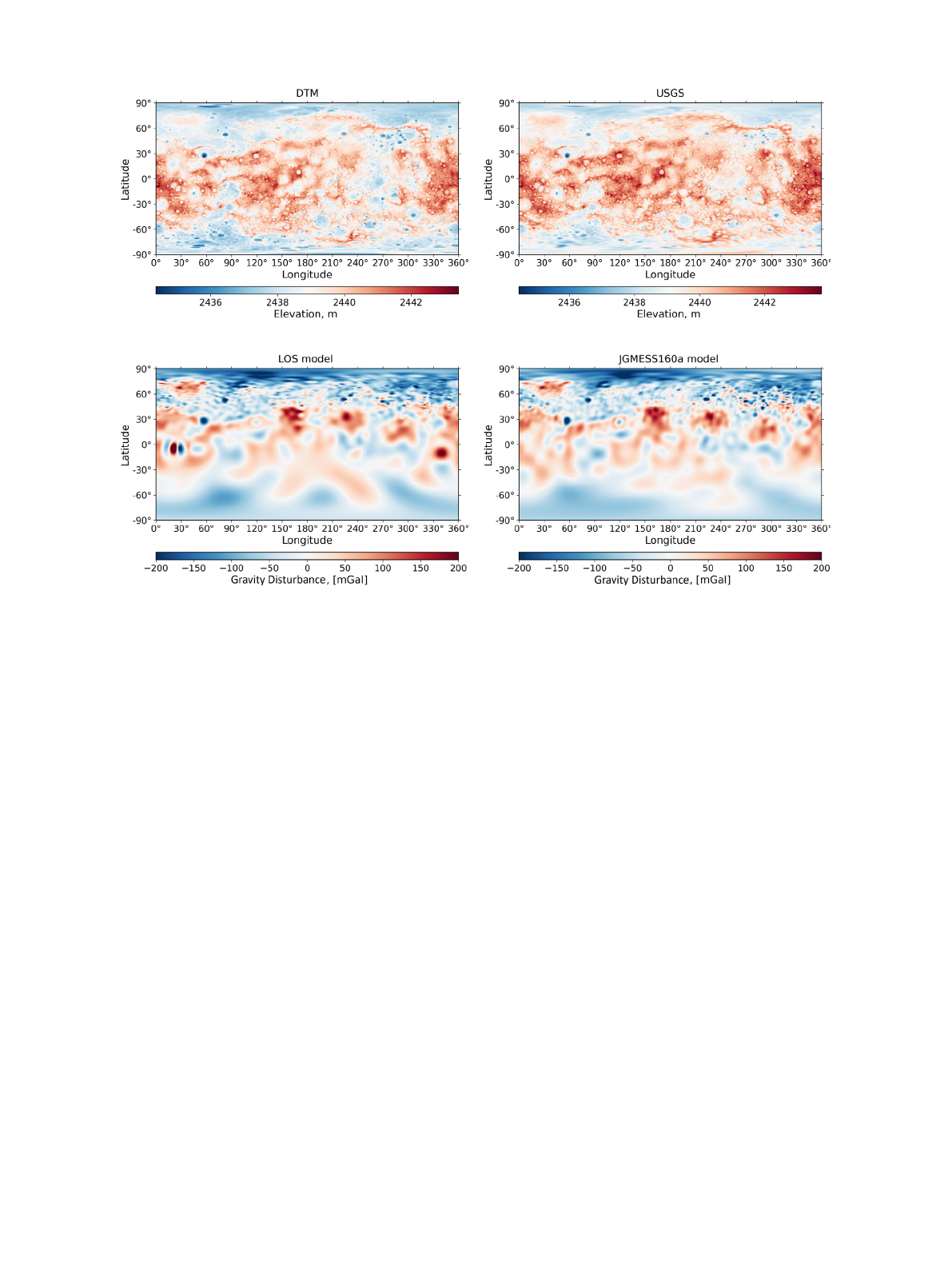
Fig. 1. Mercury’s topography and gravity field. The top shows on the left the topography DTM by Preusker et al. (2017) and on the right the USGS (Becker et al.,2016). The

figure on the bottom left shows the gravity field model determined by LOS technique by Goossens et al. (2022) up to degree and order 180 and on the right the gravity field

model JGMESS_160a (Konopliv et al.,2020) up to degree and order 160.

(V) highlight the similarities and differences of impact populations on

Mercury and the Moon.

2. Data and methods

Enhancing our understanding of the planetary crust requires ex-

amining the spatial correlation between gravity and topography data

with surface geological features such as impact craters and basins.

The comprehensive mapping of surface relief is crucial for determining

the distribution of features, while gravity anomalies provide insights

into the internal mass distribution beneath the surface. By integrating

these geophysical data sets estimations of density variations and crustal

thickness can be derived. To contribute to our knowledge of Mercury’s

crust, it is necessary to establish consistent representations of both

data, gravity and topography, coupled with surface analysis to identify

potential associations with geological structures.

The MESSENGER mission was equipped with the Mercury Dual

Imaging System (MDIS), including narrow-angle and wide-angle cam-

eras (Hawkins et al.,2007), as well as the Mercury Laser Altimeter

(MLA) for topography measurements (Cavanaugh et al.,2007). Images

from MDIS taken at low incidence angle provide global coverage for

morphological analysis. These images have been mosaiced to a global

data set (250m/px) and were used in this study for this purpose (Becker

et al.,2016;Hawkins et al.,2007;Cavanaugh et al.,2007) (Fig. 1).

MLA combined with radio occultation data allowed production of a

topography model expressed in spherical harmonics of degree and

order 150, corresponding to a spatial resolution of 25.4 km (Neumann

et al.,2016). Due to the elliptical orbit, the quality and quantity of

the laser footprints on the surface decreases constantly towards the

south (noticeably from 30 degrees north). Therefore, only the stereo

analysis of the MDIS stereo images remains in order to determine the

remaining global topography. The possibility to use the MDIS narrow-

angle camera (NAC) or the wide-angle camera (WAC) depending on

the distance to the surface allowed to cover the surface in adequate

resolution (200 m/pixel) in stereo. Using these data, the USGS pub-

lished a global surface model with a grid spacing of 64 pixels per degree

from about 12.5 million adjusted control points (Becker et al.,2016).

However, this implies that the USGS DTM consists of over 90 percent

interpolated points and therefore only has an effective resolution of

15–20 km. Furthermore, a comparison with MLA shows longwave-

length differences in elevation of up to 600 m. Therefore, we have used

high-resolution (222 m/pixel) Digital Terrain Models (DTMs), which

were produced by means of stereo-photogrammetry (Preusker et al.,

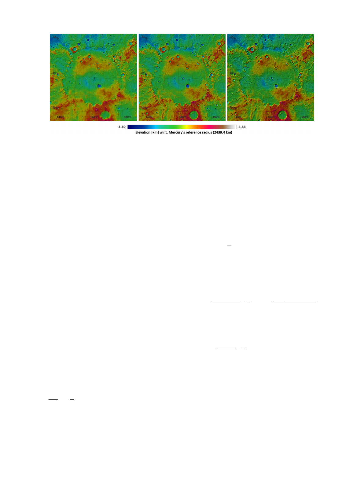
2017). These quadrangle wise produced surface models demonstrate

high geometric stability over large areas and are in a good agreement

with the MLA data (Preusker et al.,2017). As these fourteen quadrangle

DTMs among themselves and also to the MLA model do not show any

significant deviation (below 50 m), we merged these models and the

H1 quadrangle model from MLA to a high-resolution (222 m/pixel) to

a global DTM. This global DTM used in the following has the same

properties as the individual quadrangle DTMs in terms of accuracy and

stability. The percentage of interpolated points is less than 0.1 percent

and the mean point error is +/−50 m (Fig. 2). This global DTM has an

effective resolution of 2–3 km.

Starting with the MESSENGER flybys, models of Mercury’s gravity

field were refined and continuously extended in resolution as more

tracking data, especially at lower altitudes, became available. One of

the most recent gravity field model solutions is JGMESS_160a with a

resolution of degree and order 160, which is equivalent to a resolution

of approximately 23.8km in the spatial domain (Konopliv et al.,2020).

The gravity model JGMESS_160a is also lacking of details in the south-

ern hemisphere due to the eccentricity of MESSENGER’s orbit (Fig. 1).

Icarus 422 (2024) 116244

C.C. Szczech et al.

Fig. 2. Hill-shaded color-coded DTMs of the Caloris basin in stereographic (conformal) projection centered at 31◦Nand 162.5◦E. Left: MLA DTM Middle: Merged DLR DTM

(consisting of the Quadrangle DTMs H3, H4, H8 and H9.) Right: USGS DTM.

Therefore, the values of the gravity field model have a significant error

towards the south and need to be treated with caution. Compared

to the north pole region, about one order of magnitude larger error

can be assumed at the south pole. Another recent study presented a

gravity solution up to degree and order 180 using high-resolution Line-

of-sight (LOS) techniques to obtain a more detailed analysis of surface

features (Goossens et al.,2022) (Fig. 1). The gravity disturbance is

here refereed as the total gravity acceleration after the normal gravity

have been subtracted from the observed gravity without the elevation

correction (Wieczorek,2015;Wieczorek and Meschede,2018).

2.1. Gravity anomaly

Gravity anomaly refers to the difference between the observed

gravitational field strength at a specific location on the planet’s surface

and the expected gravitational field strength at that same location,

which is calculated based on a reference model (Turcotte and Schubert,

2002).

The Bouguer correction is applied, effectively removing the grav-

itational effects of surface topography and allowing us to focus on

the density variations within the subsurface (Turcotte and Schubert,

2002). The Bouguer correction compensates for the attraction of the

mass between the observation point and the reference level, taking into

account the elevation differences between the surface and the reference

level, and assuming an average crustal density of the rocks above the

reference level.

2.2. Calculating gravity anomalies and crustal thickness

The Python module SHTOOLS was used to calculated the Bouguer

anomaly (Wieczorek and Meschede,2018). We used the gravity so-

lution JGMESS_160a, which includes the measured gravity values in

spherical harmonic coefficients, and the DTM, representing the surface

elevation. We converted the DTM topography data into a set of spheri-

cal harmonics up to degree and order of 765. The spherical coordinate

expansion for spherical potential coefficients may be expressed as:

𝑈(𝑟, 𝜃, 𝜙) = 𝐺𝑀

𝑟∑

𝑖𝑙𝑚 (𝐷

𝑟)𝑙

𝐶+

𝑖𝑙𝑚𝑌𝑖𝑙𝑚(𝜃, 𝜙)(1)

with Ubeing the spherical potential, 𝜃being colatitude and 𝜙longi-

tude, Rbeing the radius, Gbeing the gravitational constant, Mbeing

the mass, 𝐶𝑖𝑙𝑚 and 𝑌𝑖𝑙𝑚 the two spherical harmonic coefficients, mand

lthe degree and order respectively (Wieczorek and Phillips,1998).

If the information on the topography and gravity observation of

a planet is provided, the method described above can be applied to

calculate both the Bouguer correction (representing the gravitational

impact of the topography) and the Bouguer anomaly (derived from

the total gravity field minus the Bouguer correction) (Wieczorek and

Phillips,1998). Further, the Bouguer anomaly can be employed to

deduce variations along an assumed density boundary beneath the

surface. However, during this process, the Bouguer anomaly must be

extended downward to reach this boundary, and this extension tends

to magnify any noise present in the data. Therefore, this method ensure

a downward continuation filter to regulate the degree of difference

between the observed and modeled field by minimization for the total

relief along this interface on a degree-by-degree basis (Wieczorek and

Phillips,1998). The combined measure of the data alignment and the

relief of the topography can be expressed as

𝛷=[𝐶𝐵𝐴

𝑖𝑙𝑚 −𝐶𝐷

𝑖𝑙𝑚 (𝐷

𝑟)𝑙]2

+𝜆(ℎ𝑖𝑙𝑚)2(2)

with 𝐶𝐵𝐴

𝑖𝑙𝑚 being the Bouguer anomaly and 𝐶𝐷

𝑖𝑙𝑚 the potential coefficients

with respect to the relief ℎ𝑖𝑙𝑚 along an interface referenced to radius D

and 𝜆being the Lagrange multiplier. By substituting the expression pro-

vided in Eq. (1) for the Bouguer anomaly, including the minimization

concerning the relief, and disregarding higher-order terms, the result is

obtained as

ℎ𝑖𝑙𝑚 =𝜔𝑙[𝐶𝐵𝐴

𝑖𝑙𝑚 𝑀(2𝑙+ 1)

4𝜋𝛥𝜌𝐷2(𝑟

𝐷)𝑙

−𝐷

𝑁

∑

𝑛=2

ℎ𝑛

𝑖𝑙𝑚

𝐷𝑛𝑛!

𝛱𝑛

𝑗=1(𝑙+4−𝑗)

(𝑙+ 3) ],(3)

with 𝛥𝜌 being the density contrast. In this expression the last term is

defining the high-order correction taking the finite amplitude of the

interface relief into account. The downward continuation filter is given

𝜔𝑙=[1 + 𝜆[𝑀(2𝑙+ 1)

4𝜋𝛥𝜌𝐷2(𝑟

𝐷)𝑙]2]−1

(4)

To match the representation of the gravity solution, we truncated

the DTM data to the same degree and order of 160 and 180. The

Bouguer anomaly is estimated by removing the Bouguer correction

from the observed gravity field. We used a mean radius of 2440 km

a flattening of 0.0009. By assuming a uniform constant density of

2800 kg/m3(Konopliv et al.,2020;Genova et al.,2019,2023) for

the crust and considering a finite-amplitude correction (Wieczorek and

Phillips,1998), the gravitational attraction caused by topography could

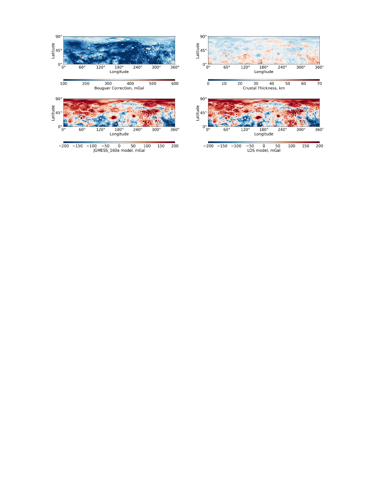
be calculated (Fig. 3).

By adding the extension ctplanet to SHTOOLS and assuming a con-

stant crustal thickness of 35 km (Beuthe et al.,2020) and porosity of

14.7% (Genova et al.,2023) we computed a map of crustal thickness for

Mercury (Fig. 3). We employed these methods to identify impact struc-

tures and their morphological features in the image and topographic

data. It facilitated the investigation of mass and density distributions,

Icarus 422 (2024) 116244

C.C. Szczech et al.

Fig. 3. Mercury’s Bouguer correction, crustal thickness and Bouguer Anomalies on the northern hemisphere. On the top left the Bouguer correction is shown, derived from the

DTM by Preusker et al. (2017). On the top right Mercury’s crustal thickness is displayed. On the bottom the Bouguer Anomalies of gravity field model JGMESS_160a (Konopliv

et al.,2020) is shown on the left and the Bouguer Anomaly of the LOS model by Goossens et al. (2022) on the right.

as well as crustal structure beneath the impact sites. However, due

to the low degree strength of the gravity models (Konopliv et al.,

2020) the gravity data is only serving as a supplementary data set

for impact structures located on the northern hemisphere, where the

degree strength is high (Fig. 3).

Comparing gravity field models derived from both standard Doppler

and LOS methods involves an evaluation of their respective strengths

and limitations. Notably, the JGMESS_160a model (Konopliv et al.,

2020) extends in spherical harmonics to degree and order 160, whereas

the LOS model expressed its resolution up to degree and order 180

(Goossens et al.,2022). The LOS method is sensitive to small-scale

features, making it suitable for geological mapping, notably impact

structures. It measures variations in the gravitational field by observing

changes in the spacecraft’s line of sight over lower altitudes (Goossens

et al.,2022). Regarding the orbit of MESSENGER, the spacecraft only

could operate in lower altitudes on the northern hemisphere. The

degree strength of JGMESS_160a varies from n=12 on the South pole

to n=154 in some regions of the northern hemisphere (Konopliv et al.,

2020). Hence, both models suffer immensely from limited resolution

towards the south. Further, the Bouguer correction is highly dependent

on the shape model. Consequently, the Bouguer anomaly may not

provide a clear representation of the underlying gravity variations in

regions with low-resolution data, as the signals are represented by

the local topographic features instead. The Bouguer signals of impact

structures, for which diameters are smaller than the degree strength

resolution are highly uncertain.

To calculate the Bouguer anomaly, a crustal density needs to be

assumed. Previous studies modeled gravity and crustal thickness assum-

ing a crustal density of 2900 kg/m3(Padovan et al.,2015;Wieczorek,

2015) and 2800 kg/m3(Genova et al.,2019;Konopliv et al.,2020;

Goossens et al.,2022). Some studies also choose a range of 2700

kg/m3to 3100 kg/m3(Konopliv et al.,2020;Beuthe et al.,2020) to

further determine crustal parameters. Some studies determined crustal

densities, such as 2957 kg/m3(Beuthe et al.,2020) 2974 kg/m3(Sori,

2018). Those need to be corrected by a rather high porosity (Beuthe

et al.,2020). Other studies determined comparable low values such

as 2600 kg/m3(Goossens et al.,2022;Genova et al.,2023). Here

we assume a standard crustal density of 2800 kg/m3, similar to the

approach of Genova et al. (2019) and Konopliv et al. (2020). The

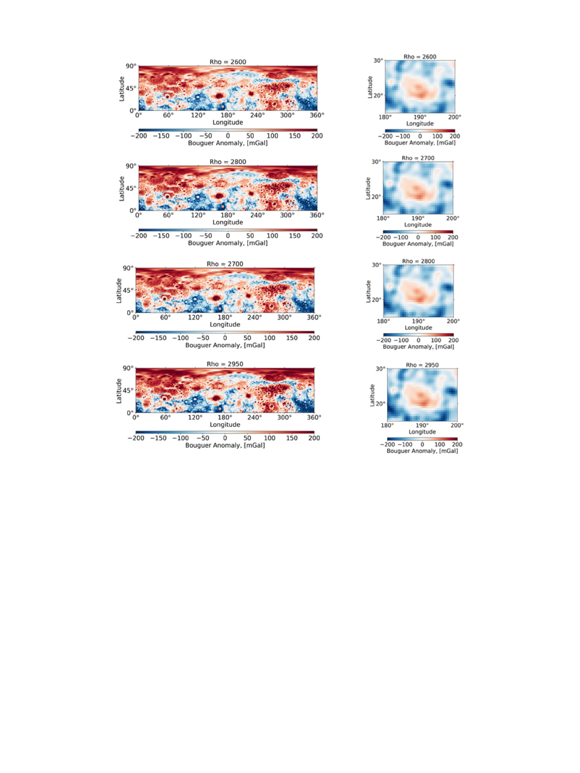
Bouguer anomalies exhibit negligible variations when using different

density values, as illustrated in (Fig. 4). Even if there is a slight

alteration in the actual Bouguer anomalies, the overarching trend of

high anomalies being situated at the center, surrounded by low values,

remains consistent. Variations in Bouguer anomaly are difficult to

interpret without any in-depth analysis. The resolution of gravity data

for Mercury is still not high enough to resolve such ambitious tasks.

2.3. Assembling the impact structure inventory: Mapping, classification and

measurements of impact structures

We use Crater Tools extension (Kneissl et al.,2011) of the geo-

graphic information system software ESRI ArcMap (ESRI 2020. ArcGIS

Desktop: Release 10.8.1 Redlands, CA: Environmental Systems Re-

search Institute), to determine crater diameters and locations from the

topographic data.

The high-resolution DTM and mosaiced satellite images provide a

clear view of the study area and impact features. The gravity data

suffer from degraded quality towards the south. It only serves as a

supplementary data set for the study. All data was examined carefully

paying close attention to variation in surface morphology, circular or

bowl-shaped depressions or gravity anomalies. Image processing was

used by enhancing the illumination and using false color schemes to

emphasize impact characteristics, such as central peaks, inner rim struc-

tures or terrain variances. Differences in variations of color, texture

and shape were visual clues to identify potential craters and basins

with diameters larger than 150 km within the data sets. The rim was

delineate of individual impact structures by tracing the circular and

bowl-shaped depressions associated with impact structures. To ensure

the accuracy and consistency of the mapped impact structures the

impact structures were re-examined and reviewed by the author and co-

authors multiple times. The mapped impact structures were compared

by previous databases for validation. Since this method is based on

subjective perception, it might be susceptible to biases.

The certainty of impact structures is based on the DTM and USGS

mosaic. Impact structures that were visible in both, topography and

Bouguer anomaly, with clear circular depression and typical morpho-

logical structures such as rim, terraces, a peak in the center or ring

structures where classified as certain basins. Whereas impact structures

that only display a circular structure in the Bouguer anomaly and low

recognition of rim features were classified as tentative suggesting buried

basins or ghost craters. Their approximated diameter was determined

by the Bouguer anomaly. Caution is advised in interpreting these

results, acknowledging potential complexities and confounding factors

due to the poor resolution of the gravity data. Yet, another origin

for these anomalies cannot be ruled out, such as gravity noise, lateral

crustal density variations or magmatic intrusions.

Icarus 422 (2024) 116244

C.C. Szczech et al.

Fig. 4. Bouguer anomaly maps using different crustal densities. On the right a close up of basin ID374 (700 km) shows the same pattern of positive Bouguer anomaly in the

center surrounded by a negative collar.

Alongside diameter and central latitude and longitude additional

attribute data was included in the catalog such as depth, gravity dis-

turbance and Bouguer anomaly of the impact structures. Using the 3D

Analyst in ArcGIS, the depth is determined as the difference in elevation

between the highest point on the rim and lowest point in the floor.

Further, these impact structures were classified into four major

classes according to the geo-morphological properties: complex craters,

central peak craters, peak ring basins, multiring basins. Impact structures

that were too modified to place into one of these categories were

cataloged separately as modified impact structures.

Gravity measurements, including gravity disturbance and Bouguer

anomaly, were taken in the central and rim areas of structures in the

gravity models by Konopliv et al. (2020) and Goossens et al. (2022).

The values were determined by the average of a single profile along 1/3

of diameter in the center of the impact structure and at the rim area.

Those profiles were chosen individually for each impact structure. Due

to limitations in resolution, signals of especially large basins seemed

irregular. From this profile the average was calculated starting from

the center to 0.33 radii and from that point to 1.33 radii.

Additionally, crustal thickness was determined for each impact

structure in the center and rim area. Since the crustal thickness map is

determined from the Bouguer anomaly, the resulting model is suffering

from the same limitations.

3. Results

We have mapped and classified a total of 314 impact structures.

297 of these are classified as certain, while 17 are classified as tentative.

we have mapped and classified a total of 314 impact structures (see

Fig. 5). Their global distribution is non-uniform, with approximately

60% of the impact structures located in the western hemisphere. This

asymmetric pattern is consistent with previous studies (Fassett et al.,

2012;Orgel et al.,2020). It could be attributed to several factors:

(I) lateral thermal variances within the crust (Orgel et al.,2020), (II)

synchronous spin and orbital periods during the planet’s early history,

transitioning to its current observed 3:2 spin–orbit resonance (Fassett

et al.,2012), and (III) resurfacing events involving the northern smooth

plains and subsequent flooding of pre-existing impact structures in the

eastern hemisphere, potentially leading to the burial of complex craters

(Byrne et al.,2016).

3.1. Mercury’s updated impact structure inventory

A catalog was established for impact structures on Mercury, includ-

ing their central latitude and longitude, diameter, depth, and character-

ization of morphology, along with gravitational properties. We provide

the inventory in Table 1 displayed in the supplementary material. A

Icarus 422 (2024) 116244

Loading more pages...