1. Introduction
The design of the VLBI global observing system (VGOS) addresses many deficiencies of its legacy system, very
long baseline interferometry (VLBI): it has small antennas that can slew between sources quickly and allow faster
sampling for better coverage of the ever-changing atmosphere, the broadband technology that increases the sensi-
tivity and the delay precision, and an instantaneous data recording system with a rate of 16 Gbps (1 Gbps=1,000
bits per second) that enables data acquisition from weaker sources (up to 250 mJy, where 1 Jy=10
−26Wm
−2
Hz
−1) and prevents the antennas from overheating (Petrachenko etal.,2009). The broadband characteristic of
VGOS and how the broadband delay is obtained allows the ionosphere contributions to be estimated more accu-
rately. Instead of using the S and X bands of geodetic VLBI systems, the broadband technology uses a range of
frequencies (2–14GHz). Coherently combining the data from these four bands and two polarizations, allows
the delay precision of single observations to be better than 16ps (1ps=10
−12 s) (Niell etal.,2018). Using this
Abstract This article focuses on the new generation of geodetic very long baseline interferometry (VLBI),
the VLBI global observing system (VGOS), and measurements carried out during the CONT17 campaign. It
uses broadband technology that increases both the number and precision of observations. These characteristics
make VGOS a suitable tool for studying the atmosphere. This study focuses on the effects of the ionosphere on
VGOS signals using a model that incorporates and extends ideas originally published in Hobiger etal. (2006,
https://doi.org/10.1029/2005RS003297). Our investigation revealed that the differential total electron content
(dTEC) data product calculated with the VGOS post-processing software had a sign error that fortunately,
does not change the final values of the phase and group delay. Therefore, this study was a way to identify
this problem within the dTEC product. After diagnosing and solving this problem, the underlying model was
modified such that instead of considering a single unknown for the latitude gradient of the ionosphere, a time
series of latitude gradients were considered that enhanced the resulting vertical total electron content (VTEC)
estimates. For evaluation purposes, time series of VTEC at each station during the CONT17 campaign were
compared with VTEC obtained from the global navigation satellite system (GNSS). The final agreement
between VGOS and GNSS was between 1.1 and 5.9 TEC units (TECU).
Plain Language Summary The ionosphere is the upper layer of the atmosphere, where free
ions and electrons bend and delay the extragalactic radio waves, which are received at ground stations. Such
radio waves can be exploited for positioning or detection of Earth's crustal movements; thus, detecting the
ionospheric effect on these signals is of paramount importance. This paper investigates the effects of this
medium on the signals emitted from celestial bodies called “quasars” and received by a system called VLBI
global observing system (VGOS) which is a new generation of very long baseline interferometry (VLBI). Being
inspired by Hobiger etal. (2006, https://doi.org/10.1029/2005RS003297), we used a station-dependent model
to estimate the temporal variation of the ionospheric total electron content (TEC). Our initial results allowed
us to correct an unreported error in the software package of VGOS, during the CONT17 campaign which we
analyzed. We also enhanced the station-dependent model so that it could achieve a better estimation of TEC.
MOTLAGHZADEH ETAL.
© 2022. The Authors.
This is an open access article under
the terms of the Creative Commons
Attribution License, which permits use,
distribution and reproduction in any
medium, provided the original work is
properly cited.
Deriving Ionospheric Total Electron Content by VLBI
Global Observing System Data Analysis During the CONT17
Campaign
Sanam Motlaghzadeh1,2 , M. Mahdi Alizadeh1,3 , Roger Cappallo4, Robert Heinkelmann3, and
Harald Schuh3,5
1Faculty of Geodesy and Geomatics Engineering, K. N. Toosi University of Technology, Tehran, Iran, 2Faculty of Science,
University of Helsinki, Helsinki, Finland, 3German Research Centre for Geosciences (GFZ), Potsdam, Germany, 4MIT
Haystack Observatory, Westford, MA, USA, 5Institute of Geodesy and Geoinformation Sciences, Technical University of
Berlin, Berlin, Germany
Key Points:
• We studied the variation of
ionospheric total electron content over
six sites as determined using data of
the new geodetic very long baseline
interferometry (VLBI) system, VLBI
global observing system (VGOS), in
December 2017
• By enhancing the model, we
estimated the temporal variation of
the latitudinal ionosphere gradient and
achieved more accurate results
• We compared our results with global
navigation satellite system vertical
total electron content which enabled
us to detect an error in the sign of
the VGOS differential total electron
content calculation
Correspondence to:
S. Motlaghzadeh,
ghodsiyehmo[email protected]i
Citation:
Motlaghzadeh, S., Alizadeh, M. M.,
Cappallo, R., Heinkelmann, R., &
Schuh, H. (2022). Deriving ionospheric
total electron content by VLBI global
observing system data analysis during
the CONT17 campaign. Radio Science,
57, e2021RS007336. https://doi.
org/10.1029/2021RS007336
Received 13 JUL 2021
Accepted 11 SEP 2022
Author Contributions:
Conceptualization: M. Mahdi Alizadeh
Data curation: Sanam Motlaghzadeh,
Roger Cappallo
Formal analysis: Sanam Motlaghzadeh
Investigation: Sanam Motlaghzadeh
Methodology: Sanam Motlaghzadeh
Resources: Roger Cappallo
Software: Sanam Motlaghzadeh
Supervision: M. Mahdi Alizadeh, Roger
Cappallo
Validation: M. Mahdi Alizadeh, Roger
Cappallo
Writing – original draft: Sanam
Motlaghzadeh
10.1029/2021RS007336
RESEARCH ARTICLE
1 of 15

Radio Science
MOTLAGHZADEH ETAL.
10.1029/2021RS007336
2 of 15
system, the baseline length estimates can be as precise as 0.3mm. For a more detailed description of the VGOS
system and its contribution to geodetic VLBI, see Niell etal.(2018).
The focal point of this paper lies in an updated way to calculate ionospheric parameters. In legacy S/X VLBI
systems utilizing X- and S-band, the differential delay caused by the ionosphere is removed by forming a linear
combination of the S and X band group delays. This procedure is done after the correlation stage. Instead, in the
VGOS data pipeline, estimates of differential total electron content (dTEC) for each baseline are made during
the correlation post-processing (Cappallo,2015). Niell etal.(2018) showed consistency between VGOS dTEC
and the differenced TEC obtained by global navigation satellite systems (GNSS) data. For legacy S/X systems
Hobiger etal.(2006) came up with a station-dependent model for estimating the frequency-dependent delay
caused by the ionosphere and thus extracting the time series of vertical total electron content (VTEC) for each of
the stations. To avoid repetition, throughout the paper, we mention this model by “the station-dependent model.”
The method described in this paper is inspired by the station-dependent model because it's not dependent on
any external data other than VLBI, but still estimates the variation of the VTEC parameter during the observing
session. Since VGOS is a new system and is in a number of ways more complex than the legacy S/X systems,
subtleties are arising from phase calibration and dTEC estimation that had to be taken into account in our analysis.
Moreover, the original station-dependent model considered only one unknown parameter for the latitude gradient
of the ionosphere. In this study, however, this assumption is enhanced by introducing a time series for ionosphere
latitude gradient. Another difference is that we used dTEC as the input data to estimate VTEC above each station
point, whereas, in the original station-dependent model, the ionospheric delay was used for this purpose.
To evaluate our result initially, the final VTEC time series are compared with VTEC from GNSS observations.
GNSS includes different satellite missions aim at positioning; namely, global positioning system (GPS), Gali-
leo, Global'naya NAvigatsionnaya Sputnikovaya Sistema (GLONASS), and BeiDou. Using a dual frequency
GNSS receiver, one can form combinations between observations and estimate the ionospheric contribution, as
it explained for example, in Hofmann-Wellenhof etal.(2001). A similar practice has been attempted with the
legacy VLBI system. In Dettmering etal.(2011), the VTEC derived from geodetic VLBI is compared to the
VTEC derived from other methods, including GNSS and the GNSS VTEC is consistent with VLBI VTEC. In this
work it is shown that the GNSS estimates have higher values than VLBI estimates, which agrees with our results.
In Sekido etal.(2003) the VTEC values derived from geodetic VLBI have been compared with global iono-
spheric map (GIM) from center of orbit determination in Europe (CODE), which is obtained from GNSS data,
and showed that there is a 90% correlation between the two data sets for the short-length baselines. Moreover,
Hobiger etal.(2006) has also made the same comparison with GIM for all VLBI sessions from 1995 to 2006 and
concluded that the overall mean difference between the two methods is −2.8 TECU which shows a good agree-
ment. He also has shown that GNSS-based VTEC is slightly higher than VLBI TEC, which matches our results.
2. Method
2.1. Extraction and Modeling of the Ionospheric Parameters
Interferometric systems such as S/X VLBI or VGOS are used to observe the difference in the interferometric
phase of a noise signal from an extragalactic radio source, as received at two different antennas. The principal
geodetic observable is group delay and according to Cappallo(2015), the correlation between group delay and
dTEC is high (more than 90%). Therefore, the precision and wide frequency coverage of the VGOS observations
necessitate accounting for the ionospheric effect at the post-correlation analysis stage. For VGOS, determin-
ing this dTEC parameter is performed by the fourfit program, which is distributed with the software package
Haystack observatory processing software (HOPS). The phase model used in this program is (Cappallo,2016):
Φ(
𝑓𝑓)=𝜏𝜏𝑔𝑔∗(𝑓𝑓−𝑓𝑓0)+Φ
0−
1.3445 ∗ dTEC
𝑓𝑓
(1)
where
𝐴𝐴Φ
is the interferometric phase (rotation),
𝐴𝐴𝐴𝐴
𝑔𝑔
is the group delay (ns), f is the frequency (GHz),
𝐴𝐴𝐴𝐴
0
is the fourfit
reference frequency (GHz),
𝐴𝐴Φ0
is the phase (rotation) at
𝐴𝐴𝐴𝐴
0
, and
𝐴𝐴dTEC
is the differential TEC (TECU=
𝐴𝐴1016
𝑚𝑚
2
).
Among other parameters, for each observation, a value for
𝐴𝐴𝐴𝐴
𝑔𝑔
and
𝐴𝐴dTEC
is estimated; this study uses those
estimates of dTEC as our raw observable. Since our raw data come from the output of the fourfit program, it is
useful to study in-depth how dTEC is retrieved.
Writing – review & editing: M. Mahdi
Alizadeh, Roger Cappallo, Robert
Heinkelmann, Harald Schuh
Radio Science
MOTLAGHZADEH ETAL.
10.1029/2021RS007336
3 of 15
The model used by the correlator has imperfectly known physical parameters, such as source and station coordi-
nates, station clock, and a non-hydrostatic part of the troposphere delay zenith wet delay. The estimates of each
parameter contain errors and thus increase the total error. As a result, there are non-zero residual delays and
delay-rates. Fringe-fitting is a post-correlation process that is responsible for correcting the errors of the estimates
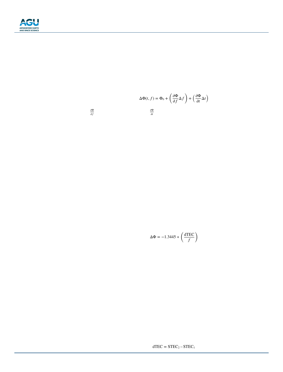
(e.g., Cotton,1995). Based on Equation1, the parameter values (dTEC and the group delay) are adjusted within
fourfit, in a manner such that all of the channel phases are as similar as possible, resulting in the greatest coherent
sum of the individual channel phasors (Cappallo etal.,2017).
Assuming small errors in the a priori parameters, the change in phase (to first order) can be written:
ΔΦ(
𝑡𝑡𝑡 𝑡𝑡)=Φ
0+
(
𝜕𝜕Φ
𝜕𝜕𝑡𝑡 Δ𝑡𝑡
)
+
(
𝜕𝜕Φ
𝜕𝜕𝑡𝑡 Δ𝑡𝑡
)
(2)
where
𝐴𝐴𝜕𝜕Φ
𝜕𝜕𝜕𝜕
is the residual group delay and
𝐴𝐴𝜕𝜕Φ
𝜕𝜕𝜕𝜕
is the residual fringe rate. Equation2 is also called the resolution
function, which is to be maximized by finding the optimal group delay and fringe rate (Rogers,1970). The opti-
mal delay and fringe rate are found through a search of coherently summed amplitudes, over a 3-dimensional
grid with axes denoting single-band delay (the group delay within each frequency channel), multi-band delay (the
group delay after tying together the phases across all frequency channels), and group delay-fringe rate (simply
delay-rate) (see, e.g., Cotton,1995). VGOS fringe fitting for an experiment requires multiple setup runs of the
program fourfit under different configurations, to correct channel phase offsets and find delay offsets for the
bands (Barrett etal.,2019). Within each scan, polarizations are coherently combined, and a fit is performed,
yielding a set of calibrated broadband VGOS observables. The independent parameters that are estimated are
interferometer phase, group delay, group delay-fringe rate, and dTEC (see Equation1) and they are adjusted such
that the coherently summed (over all channels) complex fringe amplitude is at a maximum.
Ideally, the phase calibration tones would allow the automatic adjustment of channel phases to achieve maximum
coherence. In practice, though, particularly during the early period of VGOS due to the presence of hardware
problems, it is necessary to make some “manual” adjustments to the channel phases. During the so-called manual
phase calibration, the correlator engineer picks several strong scans and determines channel-by-channel phase
offsets to maximize the fringes. Unfortunately, this has been shown to introduce small frequency-independent
phase signatures, which mimic the effect of ionospheric dispersion. In essence, each station has a small, unknown,
yet constant TEC value added to every observation. This makes it necessary to estimate and remove the effect of
this dispersion offset, as done in this research.
As shown in Equation1, the phase contribution (in radians) due to the ionosphere is:
ΔΦ = −1
.3445 ∗
(
dTEC
𝑓𝑓
)
(3)
where dTEC is the difference of TEC (in TECU) above the two stations and the phase offset is applied to each
individual frequency channel (Cappallo etal.,2017). The method used in fourfit to determine dTEC is to succes-
sively estimate the other independent parameters (phase, delay, and delay rate) at a grid of fixed values of dTEC
that span a specified range. For each trial value of dTEC, a complete fringe fit is performed and from these fits,
the interpolated maximum is found. The chosen value of dTEC (at the optimal value of delay and rate) maxi-
mizes the coherent sum of complex cross-spectral power. Note that for VGOS the cross-power spectra from the
correlator need to be combined prior to the fringe-fit. Due to the use of linearly polarized feeds, there are four
complex correlation products (XX, YY, XY, YX), which are co-added into a Stokes Intensity equivalent, taking
into account the parallactic angles of the antenna feeds (Cappallo,2016).
2.2. Formulation of the Theoretical Model
The ionosphere is a dispersive medium where signals are both refracted and delayed in a frequency-dependent
manner (Böhm and Schuh,2013). In the current study, we ignore ionospheric refraction, as well as the higher-order
terms of ionospheric delay (Hawarey etal.,2005), as they are currently below our sensitivity level.
The differential ionosphere can be treated as the difference of the TEC along the two slanted ray paths, STECi
dTEC = STEC2
–
STEC1
(4)
Radio Science
MOTLAGHZADEH ETAL.
10.1029/2021RS007336
4 of 15
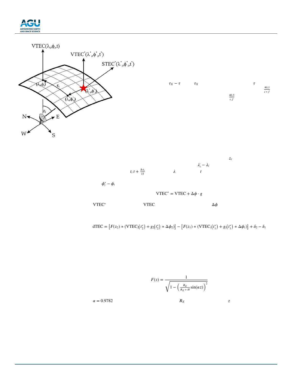
Figure 1 illustrates the single layer model (SLM) for the ionosphere
(Schaer,1999). According to this assumption, no variation in longitude is
explicitly solved for—changes in longitude only enter implicitly through the
time dependency of parameters (Dettmering etal.,2011).
The discrepancy between our work and the original station-dependent model
arises from the fact that the original station-dependent model uses the iono-
spheric delay (
𝐴𝐴𝐴𝐴
𝑋𝑋
−
𝐴𝐴
, where
𝐴𝐴𝐴𝐴
𝑋𝑋
is the total delay in X band and
𝐴𝐴𝐴𝐴
is the ionos-
pis the ionospe-free combination) dTEC using the ionospheric factor
𝐴𝐴40.3
𝑐𝑐
∗
𝑓𝑓
and
converts it to dTEC using the ionospheric factor
𝐴𝐴40.3
𝑐𝑐.𝑐𝑐
(where c is the speed of
light and f is the frequency) to estimate the VTEC values, but our fundamen-
tal datum is dTEC data and there is no need to the converting factor. More-
over, we improved the model represented in the original station-dependent
model in ways; namely by changing the definition of latitude gradient and
producing a time series for it, using a different piece-wise linear function
for generating time series, removing the non-negative constraint matrix for
estimating VTEC, and substituting the instrumental delay with the dispersion
offset (see section2-1) as an unknown parameter.
In Figure 1 quantities with * superscript refer to the ionsopheric pierce
point(IPP), the i index refers to the station and
𝐴𝐴𝐴𝐴
𝑖𝑖
is the zenith angle of the
station. The longitude offset,
𝐴𝐴𝐴𝐴
⋅
𝑖𝑖
−
𝐴𝐴𝑖𝑖
, is compensated for by changing the
observation timetag, that is,
𝐴𝐴𝐴𝐴
𝑖𝑖𝐴𝐴+
Δ𝜆𝜆
i
15
, i=1,2, where
𝐴𝐴𝐴𝐴
is in degrees,
𝐴𝐴𝐴𝐴
is in hour, and degrees and hour are related
to each other by hour=degrees/15. The gradient of TEC in latitude, -g, is solved for, and multiplied by the lati-
tude offset,
𝐴𝐴𝐴𝐴
∗
𝑖𝑖
−
𝐴𝐴𝑖𝑖
. Thus, the VTEC in IPP can be related to the VTEC in station with Equation5.
VTEC∗= VTEC + Δ𝜙𝜙
⋅
𝑔𝑔
(5)
where
𝐴𝐴VTEC∗
is the VTEC in IPP,
𝐴𝐴VTEC
is the VTEC at the station, and
𝐴𝐴Δ𝜙𝜙
is the latitude difference between
station and IPP.Based on Equation4 and considering the additional effect that is produced during the correlation
process, the observation equation now reads:
dTEC = [𝐹(𝑧
2
)∗ (VTEC
2
(𝑡∗
2)+𝑔
2
(𝑡∗
2)∗Δ𝜙
2
)]−[𝐹(𝑧
1
)∗ (VTEC
1
(𝑡∗
1)+𝑔
1
(𝑡∗
1)∗Δ𝜙
1
)]+𝛿
2
−𝛿1
(6)
where VTECi is the piece-wise linear function for VTEC, gi(t) is the piece-wise linear latitude gradient function
(in TECU/deg), δi is the dispersion offset, and F(z) is the mapping function. The dispersion offsets make the
design matrix singular, as VLBI only makes differential delay measurements; hence to resolve them, similar to
the original station-dependent model, the additional constraint is placed that the sum of all station dispersion
offsets is equal to zero. Moreover, similar to the original station-dependent model, we adopted the modified SLM
(MSLM) mapping function of the ionosphere (Schaer,1999):
𝐹𝐹
(𝑧𝑧)=
1
√
1−
(
𝑅𝑅𝐸𝐸
𝑅𝑅𝐸𝐸+𝐻𝐻sin(𝛼𝛼𝑧𝑧)
)
2
(7)
where
𝐴𝐴𝐴𝐴=0.9782
is the scaling factor, and H=506.7,
𝐴𝐴𝐴𝐴
𝐸𝐸
is the Earth radius, and
𝐴𝐴𝐴𝐴
is the zenith angle. In this
study, due to the high temporal resolution of VGOS observations which is one minute or less, each group of
15 sequential observations represents one interval, whereas in the original station-dependent model this value
was set to 8.
Our model consists of three components: for each station, there is a time series representing VTEC above that
station, another time series for the latitude gradient of VTEC, and a dispersion offset. When defining the time
series in the station-dependent model, an offset is introduced and the slope between each two data points are
estimated. This method increases the error, since by changing the offset value the whole time series will move up
or down. Instead, we implement piece-wise linear polynomials that estimate only the values of endpoints, both
for the VTEC and latitude gradient time series; the model estimates the values of the endpoints of each connected
Figure 1. Vertical total electron content (VTEC) at the ionospheric pierce
point and its relation to the VTEC on the station point (taken from Hobiger
etal.[2006]).
Radio Science
MOTLAGHZADEH ETAL.
10.1029/2021RS007336
5 of 15
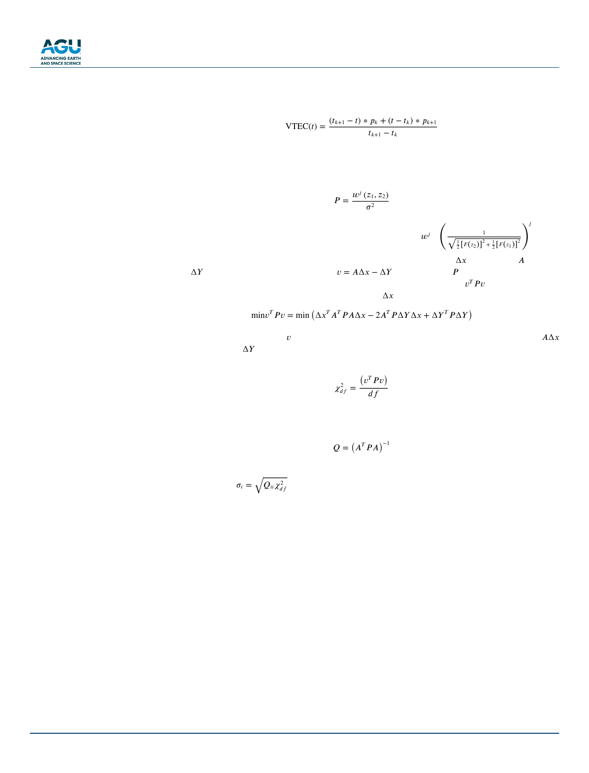
segment. Specifically, if the endpoints are a set of (n+1) values having a time tk and a rate pk, with k running
from 0 through n, when t lies in the interval [tk, tk+1] the piece-wise linear function VTEC(t) is given by:
VTEC(
𝑡𝑡)=
(𝑡𝑡
𝑘𝑘+1
−𝑡𝑡)∗𝑝𝑝
𝑘𝑘
+(𝑡𝑡−𝑡𝑡
𝑘𝑘
)∗𝑝𝑝
𝑘𝑘+1
𝑡𝑡𝑘𝑘+1 −𝑡𝑡𝑘𝑘
(8)
To perform a Least-Squares fit, we need to form a residual vector and minimize the squared sum of these resid-
uals weighted by a weight matrix. The weight matrix (P) is defined by wk which is the weight of the mapping
function divided by the error of observations (reported by the fourfit program).
𝑃𝑃
=𝑤𝑤
𝑗𝑗
(𝑧𝑧1,𝑧𝑧
2
)
𝜎𝜎
2
(9)
where σ is the vector of observations error (here dTEC formal error) and
𝐴𝐴𝐴𝐴
𝑗𝑗
is
𝐴𝐴(
1
√
1
2[𝐹𝐹(𝑧𝑧2)]2+1
2[𝐹𝐹(𝑧𝑧1)]2
)𝑗𝑗
.
According to Hobiger and Schuh(2004), the best option for j is 4. If we define the
𝐴𝐴∆𝑥𝑥
as unknowns,
𝐴𝐴𝐴𝐴
as design
matrix,
𝐴𝐴∆𝑌𝑌
as observed minus calculated vector,
𝐴𝐴𝐴𝐴=𝐴𝐴∆𝑥𝑥−∆𝑌𝑌
as residuals and
𝐴𝐴𝐴𝐴
as the weight matrix (which
is inversely proportional to the square of observations uncertainty), by minimizing
𝐴𝐴𝐴𝐴
𝑇𝑇𝑃𝑃𝐴𝐴
the problem will be
solved as seen in Equation10. The derivatives with respect to
𝐴𝐴∆𝑥𝑥
must be set to zero (Koch,1997).
min
𝑣𝑣
𝑇𝑇
𝑃𝑃𝑣𝑣= min
(
∆𝑥𝑥
𝑇𝑇
𝐴𝐴
𝑇𝑇
𝑃𝑃𝐴𝐴∆𝑥𝑥−2𝐴𝐴
𝑇𝑇
𝑃𝑃∆𝑌𝑌∆𝑥𝑥+∆𝑌𝑌
𝑇𝑇
𝑃𝑃∆𝑌𝑌
)
(10)
To ensure that the residual vector (
𝐴𝐴𝐴𝐴
) is converging, and assess the goodness-of-fit of our calculated dTEC
𝐴𝐴𝐴𝐴∆𝑥𝑥
to the observed dTEC
𝐴𝐴∆𝑌𝑌
, we used a reduced chi-square statistic or the variance of unit weight. If the statistic is
bigger than 1, the estimation procedure stops. In Equation11 one can find the statistics of reduced chi-square test.
𝜒𝜒
2
𝑑𝑑𝑑𝑑 =
(
𝑣𝑣𝑇𝑇𝑃𝑃𝑣𝑣
)
𝑑𝑑𝑑𝑑
(11)
where df is the degree of freedom (observations-unknowns). The estimations accuracy is stored in a
variance-covariance matrix, Q:
𝑄𝑄
=
(
𝐴𝐴𝑇𝑇𝑃𝑃𝐴𝐴
)−1
(12)
The final standard deviation of estimates is found by multiplying Equation11 to the diagonal elements of Q in
Equation11, that is,
𝐴𝐴𝐴𝐴
𝑖𝑖=
√
𝑄𝑄𝑖𝑖𝑖𝑖𝜒𝜒2
𝑑𝑑𝑑𝑑
(Koch,1997).
We start the processing directly with dTEC that is found in the “Observables” folder of the data in the vgosDB file
format (for more information about vgosDB format, see Gipson[2015]), alongside its formal error of about 0.04
TECU reported by the fourfit program. The analysis described above is performed using MATLAB.
3. Data and Processing
Vienna VLBI software (VieVS) was developed at the Vienna university of technology (TU Wien) using MATLAB
software and has been used extensively for analyzing VLBI data. After processing each session, a mat-structure
file is stored in which all scans are organized sequentially, from which VTEC above each station can be extracted
(Böhm etal.,2018).
For this study, we initially used VieVS to process the VGOS sessions, acquired in the CONT17 campaign (see
Behrend etal.,2020) and then, using the mat-structure file obtained by VieVS, applied the algorithm mentioned
in section2-2 for deriving VTEC and latitude gradient values from this data set. This campaign, carried out by
IVS (International VLBI Service, see Nothnagel etal.,2017), took place over a time period of about two weeks
that only about a third of which, 5days from the interval 3–8 December 2017, were observed with a VGOS broad-
band network. Principally we used data from the 3 December session to construct TEC and its latitude gradient
above each station, although other sessions were processed for comparison. The stations that participated in this
campaign were the Goddard Geophysical and Astronomical Observatory (GGAO12M), Westford (WESTFORD),
and Kokee (KOKEE12M) in the United States, Ishioka (ISHIOKA) in Japan, Yebes (RAEGYEB) in Spain, and
Loading more pages...