
Citation: Bunsen, J.; Finkbeiner, M.
An Introductory Review of
Input-Output Analysis in
Sustainability Sciences Including
Potential Implications of Aggregation.
Sustainability 2023,15, 46. https://
doi.org/10.3390/su15010046
Academic Editor: Cuihong Yang
Received: 21 November 2022
Revised: 13 December 2022
Accepted: 14 December 2022
Published: 20 December 2022
Copyright: © 2022 by the authors.
Licensee MDPI, Basel, Switzerland.
This article is an open access article
distributed under the terms and
conditions of the Creative Commons
Attribution (CC BY) license (https://
creativecommons.org/licenses/by/
4.0/).
sustainability
Article
An Introductory Review of Input-Output Analysis in
Sustainability Sciences Including Potential Implications
of Aggregation
Jonas Bunsen *,† and Matthias Finkbeiner †
Chair of Sustainable Engineering, Technische Universität Berlin, 10623 Berlin, Germany
*Correspondence: [email protected]
† Current address: Fachgebiet für Sustainable Engineering, Technische Universität Berlin, Institut für
Technischen Umweltschutz, Sekr. Z 1, Straße des 17. Juni 135, 10623 Berlin, Germany.
Abstract: Input-output analysis has become a widely established method in sustainability sciences.
It is primarily used in macroeconomic footprint analyses for allocating an economy’s externalities
among the agents in that economy based on the agents’ input-output interdependencies. However,
databases for input-output analyses are commonly compiled by aggregating data. Aggregation
of input-output data inevitably leads to a loss of information and in some instances can lead to
misinformed decision-making. The goal of this paper is to provide a simple hands-on numerical
introduction to input-output analysis including the potential implications of data aggregation in an
original manner. First, the calculation of production-based and consumption-based inventories is
introduced based on a dummy 2
×
2 input-output table. Next, the inventories of the 2
×
2 input-
output table are compared with the production-based and consumption-based inventories of a
corresponding non-aggregated 4
×
4 input-output table. A comparison of the inventories of both
dummy input-output tables allows for an exemplary demonstration of inaccurate allocation as a
result of data aggregation and to conclude on potential implications for decision-making. Overall, this
work offers a succinct and numerically substantiated introductory review of input-output analysis
for practitioners in sustainability sciences including the potential implications of aggregation of
input-output data. Its simplistic approach sets this work apart from other publications on aggregation
in input-output analysis that are founded in economics or econometrics.
Keywords: input-output analysis; methods for sustainability assessment
1. Introduction
Over the last few centuries, humanity’s footprint on planet earth has grown dra-
matically. Particularly since the middle of the 20th century, the world’s population and
its wealth have increased enormously and accompanied by an escalated anthropogenic
appropriation of the earth’s resources and exhaustion of the earth’s capacity to absorb
emissions [
1
–
3
]. It is now widely accepted that humanity’s current patterns of consumption
and production cannot be sustained without causing significant and potentially threatening
changes to the earth’s biosphere [
4
–
8
]. Consequently, individuals, organisations and entire
nations have committed to reducing their ecological footprint, as well as the entirety of
humanity’s ecological footprint. Hence, there is a need for robust methods and tools to
examine which agents in the global economy are responsible for the extraction and emission
of physical substances.
One such method is input-output analysis. Initially, input-output analysis was founded
in macroeconomics by Wassily Leontief for investigating the interdependencies between pro-
ducers and consumers based on their input-output interdependencies [
9
–
11
]. Later, Leontief
formulated how “undesirable by-products
. . .
are linked directly to the network of physical
relationships
. . .
of our economic system” and elaborated on “how such ‘externalities’ can
Sustainability 2023,15, 46. https://doi.org/10.3390/su15010046 https://www.mdpi.com/journal/sustainability

Sustainability 2023,15, 46 2 of 24
be incorporated into the [... ] input-output picture of [an] economy” [
10
]. In other words,
Leontief extended the initially macroeconomic application of input-output analysis with e.g.,
environmental or social metrics [
10
]. This expanded the scope of application of input-output
analysis to topics commonly understood as sustainability sciences.
Leontief [
10
] and Kitzes [
12
] offer concise introductions to environmental input-
output analysis. Leontief [
10
] provides a solid introduction to the basic mathematics of
environmentally-extended input-output analysis, including the derivation of the structural
matrix of an economy from a set of linear equations. A strength of Kitzes [
12
] is its straight-
forward approach and its accessibility for those without a mathematical background. Miller
and Blair [
11
] has become a standard reference for input-output analysis and elaborates
extensively on the foundations of input-output analysis, data organisation, input-output
multipliers, incorporation of environmental and social metrics into input-output analysis,
decomposition analysis and numerous other topics.
Input-output analysis has been applied in countless sustainability-related studies
e.g., on cities [
13
–
18
], organisations [
19
,
20
], economic sectors [
21
,
22
], nations [
23
–
30
], local
impacts of global trade [
26
,
31
,
32
] and other topics. The externalities analysed using input-
output analyses are versatile, and include carbon emissions [
17
,
18
,
33
], biodiversity [
34
],
land use [
35
,
36
], water consumption [
24
,
37
], human exploitation [
38
] and other indicators.
Building databases for input-output analyses involves the temporal, sectoral and
regional aggregation of source data. For instance, several products or small sectors are
typically aggregated into one large sector. Aggregation is applied if detailed information is
lacking as well as to reduce calculation requirements. The importance of aggregation in
input-output analysis has been recognised ever since and is subject to thorough scientific
debate [
9
,
10
,
39
–
41
]. A review of scientific literature on aggregation in input-output analysis
was first published by Kymn [
42
]. Fisher [
40
], Ara [
43
] and Neudecker [
44
] studied the
optimisation of aggregation for minimising the loss of information. Lenzen [
45
] elaborated
on aggregation versus disaggregation as well as on the disaggregation of environmentally
relevant sectors and Wood et al. [46] studied sectoral harmonisation.
However, most of these works are founded in economics or econometrics and target
expert practitioners of input-output analysis. However, input-ouput analysis is subject to
ever-increasing popularity in sustainability sciences. Often, sustainability scientists have
different scientific backgrounds and varying levels of technical knowledge and may not be
experts in input-output analysis.
A concise and numerical introduction to input-output analysis including the potential
implications of aggregation of input-output data for those without a strong technical back-
ground does not exist. Yet, the aggregation of input-output data and implications thereof
can potentially undermine the robustness of input-output analysis-based assessments and,
in worst-case scenarios, lead to misinformed decision-making.
Therefore, the main aim of this work is to provide an introductory review of input-
output analysis including the potential implications of aggregation of input-output data
based on numerically substantiated examples. This work aids sustainability scientists
and policymakers in betters understanding the potential implications of aggregation of
input-output data for their work.
In this work, instead of the frequently used terms environmentally-extended input-output
analysis [
12
] and environmental input-output analysis [
11
], the term input-output analysis is
used. The reason is that the former terms neglect that non-environmental externalities,
e.g., social metrics, can as well be incorporated into input-output analyses [
38
,
47
–
50
]. This
paper uses the terms direct and total intensities for monetary requirements and direct or total
externalities for the externalities that are associated with the monetary requirements.
First, a dummy 2
×
2 input-output table is introduced (Section 2.1), structural path
analysis (Section 2.2) and the calculation of production-based and consumption-based
inventories (Section 2.3) is explained. Next, a dummy 4
×
4 input-output table is gradually
introduced which serves as the hypothetical non-aggregated counterpart of the lower-
resolved 2
×
2 input-output table (Sections 2.4.1 and 2.4.2). Subsequently, the inventories

Sustainability 2023,15, 46 3 of 24
of both differently-resolved input-output tables are calculated (Section 3.4.2) and subject to
discussion (Section 4). This work concludes with a summary of the findings including the
potential implications of aggregation in input-output analysis (Section 5).
2. Method
This work expands on Kitzes [
12
] and the 2
×
2 dummy input-output table published
therein. Because this work is considered introductory, the fundamentals of input-output
analysis are covered in-depth. Equations (1)–(6) are the same as in Kitzes. However, more
in-depth explanations are given on structural path analysis, geometric series expansion and
the Leontief Inverse Matrix including explanatory depictions. Section 3shows the production-
based and consumption-based inventories of the differently resolved dummy input-output
tables, which makes possible a discussion of the differences in production-based and
consumption-based inventories, as well as the potential implications of aggregation of
input-output data.
Readers should note that the input-output table adapted from Kitzes is fictitious.
Moreover, all input-output tables in this work are a stark simplification of real input-output
tables which are significantly more complex and typically consist of thousands or ten
thousands region-sector combinations.
2.1. Input-Output Tables
Input-output tables represent the input-output characteristics of a given economy
for a specified period of time, e.g., a particular year. The represented economy could,
for example, comprise the economy of a country, the entire world, selected regions or
sub-national entities, such as that of states or provinces. Typically, an input-output table
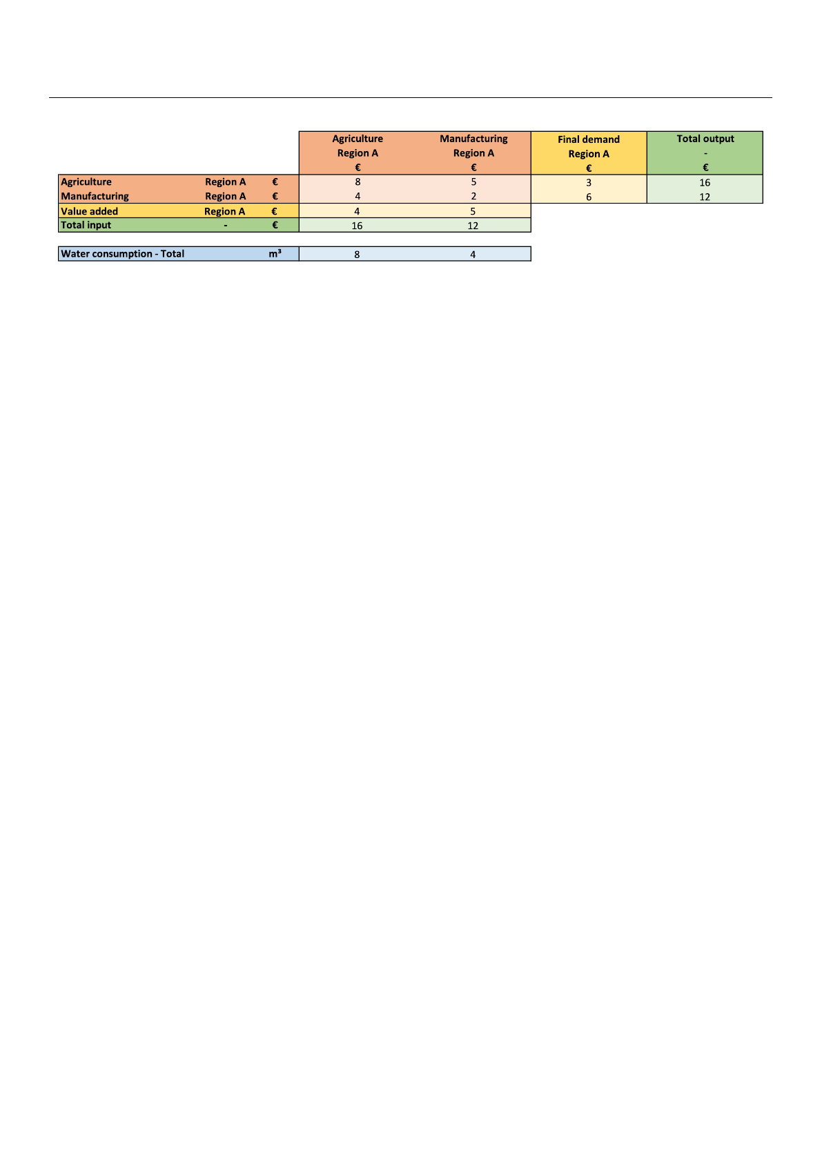
consists of the following components (see Figures 1and A1):
• Transactions (T)
• Final demand (Y)
• Value-added (V)
• Total output (xout)and total input (xin)
• Satellite accounts (Q)
The economy in the dummy input-output table in Kitzes [
12
] comprises two sectors:
Agriculture and Manufacturing (Figure 1). The rows in the transaction matrix (also known as
the Intermediate Demand Matrix) contain the sectors’ output to all other sectors (production).
For example, the Agriculture sector produces
€
8 of output for itself (intra-sectoral transac-
tion) and
€
5 of output for the Manufacturing sector (inter-sectoral transaction). In addition,
the Agriculture sector produces
€
3 of output to satisfy final demand (e.g., household con-
sumption). The total output of the Agriculture sector is
€
16. Analogously, the columns in
the transaction matrix contain the sectors’ input from all other sectors (consumption). For
example, the Manufacturing sector consumes
€
5 from the Agriculture sector and
€
2 of input
from itself. In addition, the Manufacturing sector consumes
€
5 of added value (e.g., capital
and labour). The total output of the Manufacturing sector is €12.
For sustainability assessments, input-output tables can be extended by the sectors’
externalities e.g., resource use (water, land, etc.), emissions (nitrogen, phosphorous, green-
house gases, etc.), environmental impacts (water scarcity, global warming potential, etc.),
social- (working hours, occupational fatalities, etc.) and other metrics. These extensions
are also referred to as satellite accounts (or environmental extensions). The satellite account
of the input-output table in Figure 1contains information on Water consumption—Total. It
indicates that 8 m
3
and 4 m
3
of Water consumption—Total are associated with the sectors’
total output of €16 and €12 worth of produce, respectively.
Large input-output databases are typically given in a monetary unit. The reason is
that transactions of all sorts of goods (e.g., wheat, cheese, ore, iron, cars, etc.) and services
(e.g., insurance, medical care, banking, education, etc.) in an economy can all be converted
into transactions in a common monetary unit. This allows the aggregation of thousands of
goods and services into a manageable number of aggregated sectors.
Sustainability 2023,15, 46 4 of 24
Figure 1.
Monetary 2
×
2 dummy input-output table based on Kitzes [
12
]. The sectors’ structural
paths are shown in Figure 2. The externalities per production layer are shown in
Figures 3and A2
.
The production-based and consumption-based inventories are given in Section 3.1 and shown in
Figure A3. Orange: Intra-sectoral and inter-sectoral transactions (
T
); Yellow: Value added (
V
) and
final demand (
Y
); Green: Sectors’ total input (
xin
) and sectors’ total output (
xout
); Blue: Sectors’
satellite account(s) (Q).
2.2. Structural Path Analysis
Structural path analysis refers to the systematic tracing of a sector’s inputs from all other
sectors on an infinite number of production layers based on the transaction
matrix [51–53].
A structural path can broadly be understood as a sector’s supply
chain [33,51].
Before
conducting a structural path analysis, the transaction matrix
T
and the externalities
q
are
normalised by the sectors’ total output
xout
. The normalisation yields the sectors’ input
requirements from all other sectors to produce one unit of output, also referred to as
Technical Coefficient Matrix
A
(Equation (1)), and the sectors’ externalities per one unit of
output, herein referred to as the sectors’ direct externalities
f
(Equation (2)). Consequently,
the results of the structural path analysis are given in externality per one unit of output.
A=T/xout =8 5
4 2/16 12=8/16 5/12
4/16 2/12=0.50 0.42
0.25 0.17(1)
f=q/xout =8 4/16 12=8/16 4/12=0.50 0.33(2)
In the following, an example of a structural path analysis is given. For instance, the
Agriculture sector requires inputs from itself and the Manufacturing sector. Analogously,
the Agriculture and Manufacturing sectors require inputs from sectors further up the supply
chain. In theory, this trace can be continued indefinitely. However, for sustainability
assessments a purely hierarchical description of the sectors’ structural paths is of limited
informative value. Mostly, structural paths and the quantity of an externality associated
with the respective structural path are of interest. The externalities associated with
€
1
of output from the Agriculture sector are calculated by multiplying the corresponding
direct externality
fAgriculture
by
€
1, thus yielding 0.5
m3×€
1
=
0.5
m3/€
. The externalities
associated with
€
1 of output from the Agriculture sector on the subsequent production
layers (first, second, third, etc.) are calculated by multiplying
€
1 by the corresponding
series of technical coefficients and the direct externalities of the final sector in the structural
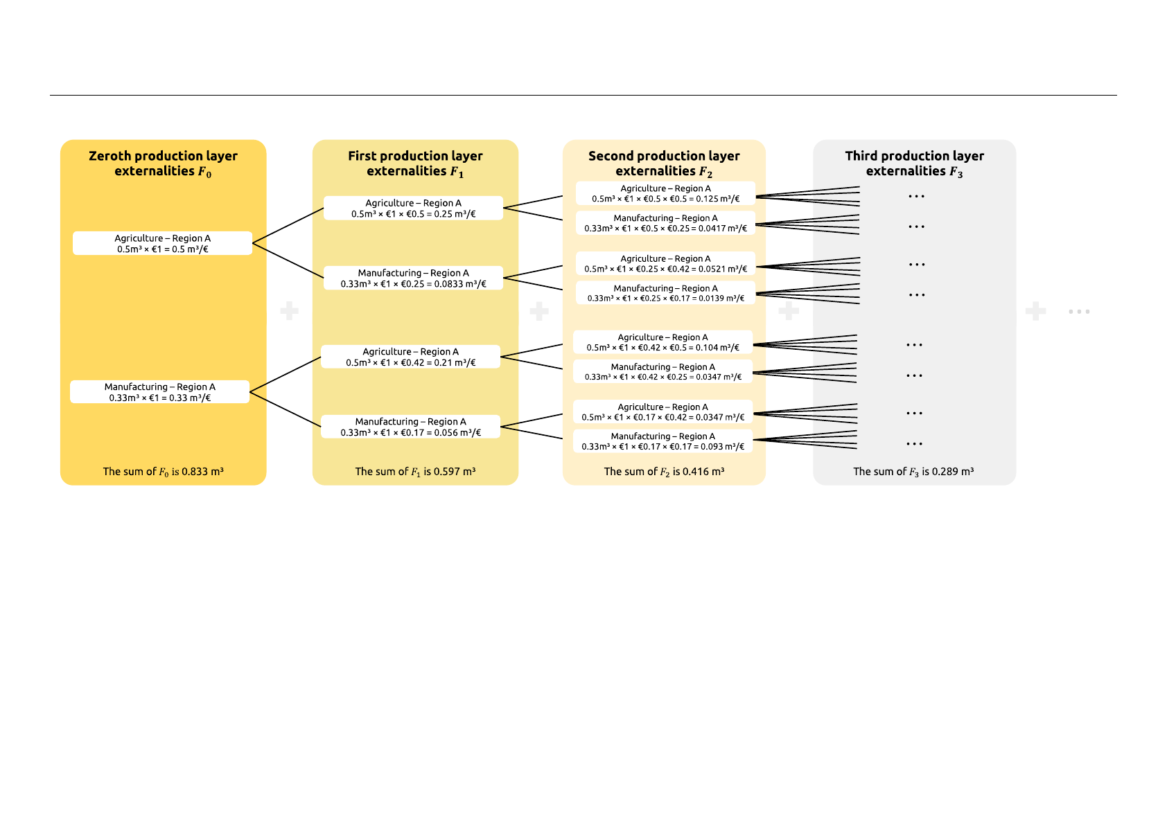
path. For example, the externalities of the Manufacturing sector on the first production layer,
the structural path Agriculture—Manufacturing, are 0.33
m3×€
1
×€
0.25
=
0.521
m3/€
. The
externalities of the Agriculture sector on the second production layer, the structural path
Agriculture—Manufacturing—Agriculture, are 0.5
m3×€
1
×€
0.25
×€
0.42
=
0.347
m3/€
(Figure 2). If this series is continued indefinitely, it becomes possible to determine a sector’s
total externalities associated with €1 of the sector’s output.
Sustainability 2023,15, 46 5 of 24
Figure 2.
Structural paths and the associated externalities of the Agriculture and Manufacturing sectors for the first three production layers (per one unit of final
demand). The totals of the externalities of a given production layer are shown at the bottom (see also Figures 3and A2).
Loading more pages...