Integrated assessment model diagnostics: key indicators and model evolution [original]

Environ. Res. Lett. 16 (2021) 054046 https://doi.org/10.1088/1748-9326/abf964

OPEN ACCESS

RECEIVED

23 December 2020

REVISED

25 March 2021

ACCEPTED FOR PUBLICATION

19 April 2021

PUBLISHED

10 May 2021

Original content from

this work may be used

under the terms of the

Creative Commons

Attribution 4.0 licence.

Any further distribution

of this work must

maintain attribution to

the author(s) and the title

of the work, journal

citation and DOI.

LETTER

Integrated assessment model diagnostics: key indicators and

model evolution

Mathijs Harmsen1,2, Elmar Kriegler3,21, Detlef P van Vuuren1,2, Kaj-Ivar van der Wijst1,2,

Gunnar Luderer3,20, Ryna Cui4, Olivier Dessens5, Laurent Drouet6, Johannes Emmerling6,

Jennifer Faye Morris7, Florian Fosse8, Dimitris Fragkiadakis9, Kostas Fragkiadakis9,

Panagiotis Fragkos9, Oliver Fricko10, Shinichiro Fujimori11, David Gernaat1,2, Céline Guivarch12,

Gokul Iyer13, Panagiotis Karkatsoulis9, Ilkka Keppo14, Kimon Keramidas8, Alexandre Köberle15,

Peter Kolp10, Volker Krey10, Christoph Krüger1,2, Florian Leblanc12, Shivika Mittal15,

Sergey Paltsev7, Pedro Rochedo16, Bas J van Ruijven10, Ronald D Sands17, Fuminori Sano18,

Jessica Strefler3, Eveline Vasquez Arroyo16, Kenichi Wada18 and Behnam Zakeri10,19

1PBL Netherlands Environmental Assessment Agency, Bezuidenhoutseweg 30, 2594 AV The Hague, The Netherlands

2Copernicus Institute for Sustainable Development, Utrecht University, Princetonlaan 8a, 3584 CB Utrecht, The Netherlands

3Potsdam Institute for Climate Impact Research (PIK), Member of the Leibniz Association, Potsdam D-14412, Germany

4Center for Global Sustainability, University of Maryland, 3101 Van Munching Hall, College Park, MD 20742, United States of America

5University College London, London, United Kingdom

6RFF-CMCC European Institute on Economics and the Environment (EIEE), Centro Euro-Mediterraneo sui Cambiamenti Climatici,

Via Bergogne 34, 20144 Milan, Italy

7MIT Joint Program on the Science and Policy of Global Change, Massachusetts Institute of Technology, Cambridge, MA, United States

of America

8European Commission, Joint Research Centre, Seville, Spain

9E3Modelling S.A., Panormou 70-72, Athens, Greece

10 International Institute for Applied Systems Analysis, Schlossplatz-1, A-2361 Laxenburg, Austria

11 Department of Environmental Engineering, Kyoto University, Kyoto, Japan & National Institute for Environmental Studies, Center

for Social and Environmental Systems Research, Tsukuba, Ibaraki 305-8506, Japan

12 Ecole des Ponts ParisTech, CIRED, 45bis avenue de la Belle Gabrielle, Nogent-sur-Marne, France

13 Joint Global Change Research Institute, Pacific Northwest National Laboratory and University of Maryland, 5825 University Research

Court, Suite 3500, College Park, MD 20740, United States of America

14 Department of Mechanical Engineering, School of Engineering, Aalto University, Otakaari 4, Espoo 02150, Finland

15 Grantham Institute, Imperial College London, Exhibition Road, London SW7 2AZ

16 Energy Planning Program, COPPE, Universidade Federal do Rio de Janeiro (UFRJ), PO Box 68565, 21941-914 Rio de Janeiro, RJ,

Brazil

17 USDA Economic Research Service, Kansas City, MO, United States of America

18 Research Institute of Innovative Technology for the Earth (RITE), 9-2, Kizugawadai, Kizugawa-Shi, Kyoto 619-0292, Japan

19 Sustainable Energy Planning Research Group, Aalborg University, A. C. Meyers Vnge 15, Copenhagen 2450, Denmark

20 Global Energy Systems Analysis, Technische Universität Berlin, Straße des 17. Juni 135, Berlin 10623, Germany

21 Faculty of Economics and Social Sciences, University of Potsdam, August-Bebel-Str. 89, Potsdam 14482, Germany

E-mail: mathijs.har[email protected]

Keywords: diagnostics, integrated assessment models, climate policy, 6th Assessment Report IPCC, renewable energy, mitigation, AR6

Supplementary material for this article is available online

Abstract

Integrated assessment models (IAMs) form a prime tool in informing about climate mitigation

strategies. Diagnostic indicators that allow comparison across these models can help describe and

explain differences in model projections. This increases transparency and comparability. Earlier,

the IAM community has developed an approach to diagnose models (Kriegler (2015 Technol.

Forecast. Soc. Change 90 45–61)). Here we build on this, by proposing a selected set of well-defined

indicators as a community standard, to systematically and routinely assess IAM behaviour, similar

to metrics used for other modeling communities such as climate models. These indicators are the

relative abatement index, emission reduction type index, inertia timescale, fossil fuel reduction,

transformation index and cost per abatement value. We apply the approach to 17 IAMs, assessing

both older as well as their latest versions, as applied in the IPCC 6th Assessment Report.

Environ. Res. Lett. 16 (2021) 054046 M Harmsen et al

The study shows that the approach can be easily applied and used to indentify key differences

between models and model versions. Moreover, we demonstrate that this comparison helps to link

model behavior to model characteristics and assumptions. We show that together, the set of six

indicators can provide useful indication of the main traits of the model and can roughly indicate

the general model behavior. The results also show that there is often a considerable spread across

the models. Interestingly, the diagnostic values often change for different model versions, but there

does not seem to be a distinct trend.

1. Introduction

Integrated assessment models (IAMs) are widely

used for climate policy and climate change ana-

lysis (van Beek et al 2020). They offer the means to

assess the linkages between long-term climate policy

goals and near-term policy choices. They can also

look into mitigation strategies taking into account

cross-sectoral and, cross-regional and systems inter-

actions (energy, land, economy, climate). As such,

they form a key information source feeding into

the climate change mitigation policy process, e.g. via

IPCC Assessment Reports (ARs) (Halsnæs et al 2000,

IPCC 2014). Within IAMs, a distinction can be made

between cost-benefit IAMs (mostly highly stylized)

and detailed process IAMs that are mostly used to

explore different pathways to reach selected policy

goals. The latter comprise a diverse group of models

with different functional structures.

A thorough understanding of how IAM struc-

ture and assumptions affect IAM behavior is critic-

ally important for assessing IAM based policy analysis

and advice. For both policy makers and researchers,

it can provide insights into why results differ between

models and link projections to policy-relevant model

assumptions and structure. It is the goal of diagnostic

tools to foster such understanding. In fact, such tools

can serve key functions: (a) characterizing model

behavior by use of stylized diagnostic experiments,

and (b) relating model behavior patterns to model

structure and input assumptions. We focus mostly on

the first in this study, but aim to cover the second,

where possible. A subsequent function, but beyond

the limits of this study is to qualify the model beha-

vior and assess models’ policy applicability.

In other modeling disciplines, similar diagnostic

tools have been developed. For instance, in climate

research, diagnostic metrics have been applied to

compare climate models and to evaluate their per-

formance (Andrews et al 2012, Flato et al 2013, Eyring

et al 2016). Such indicators, for instance, include cli-

mate sensitivity (indicating the temperature increase

for a doubling of the CO2concentration) and the

transient climate response (indicating warming over

a more limited time period). These tools are not only

used to regularly compare models and thus qualify

their behavior, but even in validation experiments,

leading to assessment of the quality of models for spe-

cific experiments and their evaluation over time.

Also the IAM community has undertaken sev-

eral model diagnostic activities in the past (Gaskins

and Weyant 1993, Weyant 2004,2010, van Vuuren

et al 2009, Wilkerson et al 2015) resulting in the most

recent and comprehensive diagnostic assessment by

Kriegler et al (2015). Here, we propose an updated

and expanded set of widely applicable, key diagnostic

indicators to be used as a community standard.

We determined these by revisiting the approach by

Kriegler et al (2015) and improving them in terms

of precision, simplicity and completeness. In partic-

ular, we propose a novel, standardized approach to

compare different model versions to assess and mon-

itor model differences over time. The approach is ana-

logous to the climate model diagnostics in the sense

that they are based on stylized scenarios with exogen-

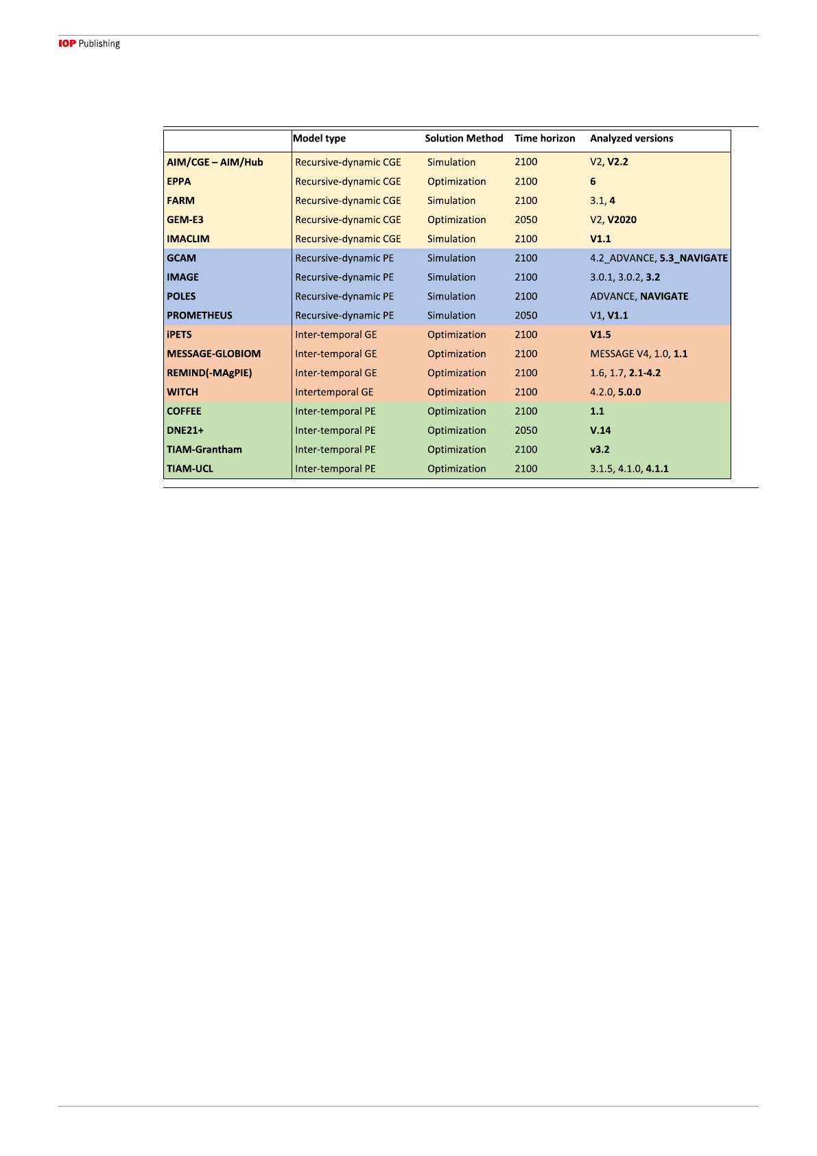
ous assumptions. It has been tested on 17 IAMs and

32 model versions, as part of two EU model devel-

opment projects, ADVANCE (www.fp7-advance.eu/)

and NAVIGATE (https://navigate-h2020.eu/), thus

providing coverage of all main process-based IAMs

(and much higher than in preceding studies), includ-

ing all latest model versions. Especially the latter is

highly needed in light of the forthcoming AR6.

A standard set of diagnostics for the community

has obvious advantages. It provides a tool to system-

atically and consistently assess model behavior in all

future studies. Model diagnostic results can be part

of model documentation that can be referenced and

highlighted in papers. Future model-intercomparison

projects could require participating models to reg-

ularly run the core set of diagnostics, to analyze

model behavior of newly developed models or model

versions. Ultimately, this will lead to greater trans-

parency and comprehensibility of IAM applications,

together with model documentation. It will also allow

tracking the development of IAMs over time—and

possibly, in the future, confronting the outcomes with

empirical information or information from other sci-

ence disciplines.

An important innovation of the present study is

the introduction of two diagnostic indicators in addi-

tion to the ones established by Kriegler et al (2015),

namely inertia timescale (IT) and fossil fuel reduc-

tion (FFR). IT provides a measure of the models’ level

of inertia in response to the introduction of climate

policy, a crucial determining factor in deep mitiga-

tion projections. FFR highlights the models tendency

to reduce fossil fuels as part of climate policy, a key

Environ. Res. Lett. 16 (2021) 054046 M Harmsen et al

element in model studies that examine the energy

transition.

Here, we present the results for six key indicators,

adding IT and FFR to the original set of indicators

from Kriegler et al (2015); relative abatement index

(RAI), carbon intensity over energy intensity (CoEI),

transformation index (TI) and cost per abatement

value (CAV). The indicators have been simplified to

make them more suitable to be used as a community

standard, namely with a focus on one strong mitig-

ation case and one benchmark year, 30 years in the

future (here 2050, but later in post-2020 assessments).

The latter allows for comparability with future dia-

gnostic assessments. To ensure precision in the dia-

gnostic results, we define single, unique values to

indicate model behavior.

In method section 2, we explain the study design

and list the participating models. The results are split-

up in subsections for each of the indicators and con-

clude with an overview table to classify all the par-

ticipating models. In the section 4, we reflect on

the research questions: Can these indicators be eas-

ily used as diagnostic tools for IAMs, including their

development over time? And what insights do these tools

provide?

2. Methods

2.1. Diagnostic experiments and indicators

The experiments described in this study form a small

selection from a larger set of stylized, diagnostic scen-

arios that have originally been developed as part of

the EU FP7 ADVANCE project (www.fp7-advance.

eu/). These are: Base (a zero carbon tax, i.e. a no-

climate policy baseline) and C80-gr5 (a run with

an exponential carbon equivalent price growth of

5% per year starting in 2020 and a price level of

80 (2010)$/tCO2eq. reached in 2040). C80-gr5 is

used for each key indicator presented here. For

two indicators (RAI and IT) extra scenarios were

used, as will be explained in the next section. Note

that the C80-gr5 scenario represents a 1.5–2 degree

case in most models (see supplement S7 (available

online at stacks.iop.org/ERL/16/054046/mmedia)),

in line with the Paris agreement’s climate ambi-

tions. This makes it a highly relevant showcase for

assessing model behavior in frequent deep mitiga-

tion scenarios. Preferably, model groups used SSP2,

the middle-of-the-road socioeconomic projection

baseline scenario (Riahi et al 2017) for all assump-

tions, including population and economic growth.

The indicators are originally chosen and adapted

here based on criteria set by Kriegler et al (2015):

•Identification of heterogeneity in model responses

•Diagnosis of relevant features for climate policy

analysis

•Applicability to diverse models

•Accessibility and ease of use

Here, we add the following criteria:

•Standardization and comparability between dia-

gnostic studies

•Precision/quantifiability

Based on these criteria, we derive a set of six

indictors that describe model responses to climate

policy. These indicators go beyond the work of

Kriegler et al, because we provide a standardized

formulation—in each case leading to a single value

that characterizes the model. We specify set rules

(benchmark year, scenario used, socio-economic

assumptions) to allow for comparability between

studies in a quantitative way. The main focus is on the

year 2050 as it is (a) policy relevant and (b) provides

a reasonable indication of model behavior through-

out the century. For future use of the indicators, we

define all indicators based on C80-gr5, using the value

30 years after the introduction of the tax (here 2020).

While the focus is on 2050, we also show the 2100 res-

ults in the supplement (S3) to assess if the 2100 num-

bers would lead to different conclusions.

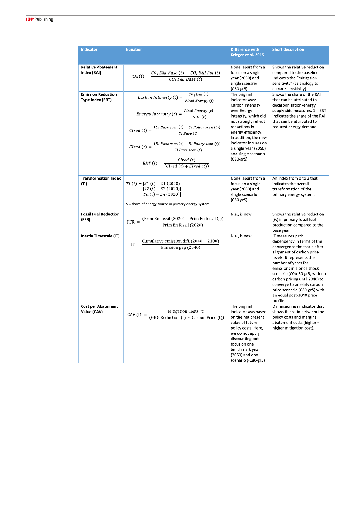
Table 1gives an overview of the key diagnostic

indicators proposed and assessed in this study. Below,

we shortly summarize the setup and rationale behind

the indicators and particularly indicate differences

with and additions to the Kriegler et al (2015)

approach. The combination of the indicators, focuses

on (a) the responsiveness of the model, (b) the type of

mitigation, (c) the scale of the transformation of the

energy system, and (d) mitigation costs as a function

of the carbon price signal.

As in earlier diagnostic exercises, the indicators

are based on global totals to assess the overall behavior

related to global climate policy. A regional assessment

would be possible in a follow-up study. All emis-

sion indicators are based on CO2energy and indus-

trial process (E&I) emissions. This allows for all mod-

els to participate (the land-use system and non-CO2

emissions are modeled by about half of the models).

Moreover, CO2E&I makes out more than two thirds

of all GHG emissions (Olivier and Peters 2020).

The RAI characterizes the emission reductions in

a carbon tax scenario relative to the baseline. It can

be considered the main indicator in the sense that

it measures the overall response to a climate policy

incentive and correlates with elements from the other

indicators (demand and supply side emission reduc-

tions, transformation rate, FFRs and limited inertia).

Hence, it can also be considered a ‘mitigation sens-

itivity’ indicator, analogous to the ‘climate sensitiv-

ity’ in climate models. In order to assess mitigation of

the full suite of GHGs, we also provide a full Kyoto

GHG analysis in the supplement (S4). In addition, an

additional scenario (C30-gr5, with a two thirds lower

tax) is used to visualize a stylized ‘derived MAC curve’

from the RAI, by connecting the projected relative

abatement at ∼0, 50 and 130 $/tCO2.

Environ. Res. Lett. 16 (2021) 054046 M Harmsen et al

Table 1. Key diagnostic indicators. For further explanation, see main text.

The ERT indicates the share of supply side meas-

ures (e.g. renewable energy) in bringing down emis-

sions. 1 minus ERT shows the share of the RAI

that that can be attributed to reduced final energy

demand. Values higher than 0.5 imply supply mod-

els (=most common), lower than 0.5 imply demand

models. This indicator replaces the CoEI indicator

from Kriegler et al 2015): CI (as a fraction of CI in

the baseline) over energy intensity, which did not

strongly reflect reductions in energy intensity (e.g. a

model with no energy efficiency at all could still be

classified as a demand focused model).

Two energy system transformation indicators

have been assessed: FFR, which is new in this study

and transformation index (TI, from Kriegler et al

2015). FFR is a simple, policy relevant indicator that

shows the relative reduction of fossil energy compared

to the base year (2020). The FFR indicator was

added to the transformation analysis, since it repres-

ents a less abstract alternative to TI and relates dir-

ectly to recent studies aimed at fossil fuel phase out

and renewable integration (in in the result section,

we also compare FFR to TI to understand what

drives transitions in models). TI shows the extent

of transformation in the energy system (2 =max,

0=none). Note that in table 1, the shares of energy

sources in primary energy system (S), are based

on the following aggregated energy sources: fossil,

Environ. Res. Lett. 16 (2021) 054046 M Harmsen et al

Table 2. Participating models, types and versions. Latest model version indicated in bold. For detailed model documentation see:

www.iamcdocumentation.eu/(IAMC wiki). See supplement (S1) for an overview of all scenarios and submissions by the different

models.

non-bioenergy renewables, bioenergy, nuclear, since

these are reported by all models, thus allowing for a

complete comparison.

In this study, we adopt a new indicator that

describes the level of inertia (i.e. persistence of path

dependency) in the models: IT. Path dependencies are

of particularly relevance for the energy system, due to

long-lived capital stocks, technological learning, and

other sources of inertia in the upscaling of new tech-

nologies, as well as behavioral inertia on the demand

side. They are also highly policy-relevant in the con-

text of delayed climate policy adoption and carbon

lock-in, as analyzed in several scenario studies (Riahi

et al 2015, Luderer et al 2018). We here introduce

a new diagnostic indicator that captures inertia in

response to the introduction of climate policy as a

crucial characteristic of IAMs. It is based on a newly

introduced diagnostic carbon price shock scenario to

quantify model representation of inertia. In our scen-

ario set, the shock scenario follows baseline develop-

ments with zero carbon prices until 2040, followed by

an instantaneous carbon price of 80$/tCO2in 2040, as

in the default scenario, with an exponentially grow-

ing carbon price thereafter. For the shock scenarios,

models with perfect foresight were instructed to dis-

able the anticipation of future carbon pricing. The

difference between the shock scenario and the default

scenario can be measured in terms of the 2040 ‘emis-

sions gap’. After 2040, the shock scenarios and cor-

responding early pricing scenarios can be expected to

converge, since they are subject to the same carbon

prices. However, during a transition period, the shock

scenarios will continue to have higher emission levels

than the corresponding early pricing scenarios, due

to the systems inertia. The IT (in units of years) is

defined as the ratio between the cumulative emission

difference between the two scenarios after 2040, and

the ‘emissions gap’ in the model year prior to 2040.

For more information and visualization see supple-

ment (S2).

The CAV is a dimensionless measure of economic

implications of emissions abatement at a certain car-

bon price. It shows the ratio between the policy costs

and marginal abatement costs (MACs). For PE mod-

els, this can be seen as an indicator for the shape

of the (implicit) MAC curve. The closer to 1 this

indicator is, the more concave the MAC curve and

the higher the projected policy costs. In other words, a

low value indicates more mitigation potential at lower

carbon prices. For GE models, macro-economic feed-

backs are also factored in. Here, a value higher than

1 implies that these feedbacks are a dominant factor

in the costs. We simplified the original indicator

by looking at a benchmark year (2050) instead of

discounting to a net present value. Note that for this

indicator, we include all greenhouse gases represen-

ted by the models (this differs per model), since that

corresponds with the model’s projected policy costs.

Reported policy cost metrics also differ per model

type. We used consumption loss compared to the

baseline for all GE models and area under the MAC

for all PE models, except for PROMETHEUS and

TIAM-Grantham where the additional total energy

system costs were applied. Although the metrics dif-

fer, they are comparable in the sense that they (at

least) factor in first-order economic expenditures,

Loading more pages...