Convergence of Discrete Period Matrices and Discrete Holomorphic Integrals for Ramified Coverings of the Riemann Sphere [original]

https://doi.org/10.1007/s11040-021-09394-2

Convergence of Discrete Period Matrices and Discrete

Holomorphic Integrals for Ramiﬁed Coverings

of the Riemann Sphere

Alexander I. Bobenko1·Ulrike B¨

ucking2

Received: 3 September 2020 / Accepted: 1 June 2021 /

©The Author(s) 2021

Abstract

We consider the class of compact Riemann surfaces which are ramified coverings of

the Riemann sphere ˆ

C. Based on a triangulation of this covering we define discrete

(multivalued) harmonic and holomorphic functions. We prove that the corresponding

discrete period matrices converge to their continuous counterparts. In order to achieve

an error estimate, which is linear in the maximal edge length of the triangles, we

suitably adapt the triangulations in a neighborhood of every branch point. Finally, we

also prove a convergence result for discrete holomorphic integrals for our adapted

triangulations of the ramified covering.

Keywords Discrete analytic function ·Riemann surface ·Period matrix ·

Discrete holomorphic integral ·Dirichlet energy ·Approximation

Mathematics Subject Classiﬁcation (2010) Primary 39A12 ·65M60 ·30E10;

Secondary 14K20 ·30F30

1 Introduction

Smooth holomorphic functions can be characterized in different ways. In particular,

the real and imaginary part of any holomorphic function is harmonic and both are

Communicated by: F W Nijhoff

Ulrike B¨ucking

[email protected]berlin.de

Alexander I. Bobenko

[email protected]berlin.de

1Institut f¨ur Mathematik, Technische Universit¨

at Berlin, Straße des 17. Juni 136, 10623,

Berlin, Germany

2Institut f¨ur Mathematik, Freie Universit¨

at Berlin, Arnimallee 3, 14195, Berlin, Germany

Published online: 2 July 2021

Math Phys Anal Geom (2021) 24: 23

related by the Cauchy-Riemann equations. This perspective naturally led to linear

discretizations of harmonic and holomorphic functions, starting with results for

square grids, see [12,14,23]. Lelong-Ferrand further developed this theory of

discrete harmonic and holomorphic functions in [19,25]. MacNeal and Duffin

generalized these notions in [15–17,27]. In particular, they considered arbitrary tri-

angulations in the plane and discovered the cotan-weights. The cotan-Laplacian is

also considered for triangle meshes, for example for surfaces in discrete differential

geometry, see [35], or for applications in computer graphics, see for example [32].

Further properties and theorems of the smooth theory of holomorphic functions have

found recently discrete analogues in the discrete linear theory in [2,3].

Note that there are other important nonlinear discretizations of holomorphic func-

tions, for example involving circle packings or circle patterns [8,9,36,38], connected

to cross-ratios [6,28], using discrete conformal equivalence [1,10], or based on bi-

colored triangles [18,34]. The linear theory of holomorphic functions on rhombic

lattices can be obtained as infinitesimal deformation of circle patterns [5].

Mercat generalized in [29] the discrete linear theory from planar subsets to discrete

Riemann surfaces and introduced in [30,31] discrete period matrices. In [4] numer-

ical experiments are considered to compute discrete period matrices for polyhedral

surfaces explicitly and compare them to known period matrices for the correspond-

ing smooth surfaces. A convergence proof for the class of polyhedral surfaces was

obtained in [7].

The interest in numerical computation of period matrices is for example motivated

by the computation of finite-genus solutions of integrable differential equations. As

Riemann surfaces may be represented as algebraic curves, this is often taken as a

starting point for computing discrete period matrices. Recent results in this context

include [13,20–22,33].

In this article, we take a different approach and consider Riemann surfaces which

are ramified coverings of the Riemann sphere ˆ

C. Based on a triangulation of this cov-

ering discrete period matrices can be obtained from this discrete data. Furthermore,

we prove convergence of the discrete period matrices to their continuous counterparts

(Theorem 3). In particular, we obtain an error estimate, which is linear in the maxi-

mal edge length of the triangles if we adapt the triangulations in a neighborhood of

every branch point. The details of our ‘adapted triangulations’ will be explained in

Section 2.3.

The convergence of discrete analytic functions to their continuous counterparts

remains an important issue, although several results have been proved by now. In par-

ticular, for the linear theory, convergence was first shown for the square lattice [12,

25]and recently for more general quadrilateral lattices [7,11,37]. In this article,

we prove the convergence of discrete holomorphic integrals (Abelian integrals of

first kind) obtained from suitable triangulations of the ramified covering to their

continuous counterparts (Theorem 4).

Our main results are stated in Section 2andprovedinSection3. The proof is

inspired by [7] and uses energy estimates which allow to prove the convergence of

the discrete period matrices directly. Our results are also applied to improve the con-

vergence results of [7] in Section 5. Finally, in Section 6, we present some numerical

experiments.

23 Page 2 of 30 Math Phys Anal Geom (2021) 24: 23

2 Convergence Results for Discrete Period Matrices and Discrete

Holomorphic Integrals for Ramiﬁed Coverings of ˆ

In the following, we consider any compact Riemann surface Rof genus g⩾1which

allows a branched covering map f:R→ˆ

C. Using this covering map as a local

chart, we always locally identify points in Rwith their images in ˆ

C. Then for points

in the complex plane C=ˆ

C\{∞}we use the standard complex coordinate z.This

map from Rto Cis denoted by Pr

Rand gives a local chart in a neighborhood about

every point, except at branch points and infinity. For further use, we fix a radius ρ>1

such that the images of all branch points, except possibly ∞,haveadistanceatmost

ρ/2 from the origin. In order to consider a neighborhood of infinity, we consider a

second chart with the local coordinate 1/z. This map from Rto Cis denoted by

Pr∞

Let T=TRbe a triangulation of Rsuch that all branch points are vertices. We

assume that every triangle is contained in only one sheet of the covering. We will

mostly consider this triangulation via its (local) image under the charts Pr

Rand

Pr∞

R. In this sense, without further mention, we always identify this triangulation

with the corresponding (multi-sheeted) triangulation on ˆ

C(which is the image f(T)

under the covering map) and with the (multi-sheeted) image of this triangulation of ˆ

under the charts Pr

Rand Pr∞

R. We assume that this triangulation is a locally planar

embedding in the complex plane Cor equivalently in the Riemann sphere ˆ

C, except at

the branch points. From now on, we consider the vertices of the triangulation as points

of C, that is, we always apply the local charts Pr

Rand Pr∞

R. The edges connecting

incident vertices will be straight line segments or circular arcs in C, depending on the

following distinction.

(i) All triangles whose images under the chart Pr

Rhave at least two vertices in

the open disc Bρ(0)of radius ρabout the origin are geodesic, that is Euclidean

triangles. We always consider these triangles to be embedded in C.

(ii) All triangles whose image under the chart Pr∞

Rhave all vertices contained in

the closed disc B1/ρ(0)of radius 1/ρ about the origin (that is, in the images

under the chart Pr

Rall vertices are contained in the complement C\Bρ(0))

are geodesic, that is Euclidean triangles. We always consider these triangles to

be embedded in C. Note that in the image under the chart Pr

Rthese triangles

are preimages of a geodesic triangulation with Euclidean triangles under the

map z→ 1/z. Therefore, these triangles are in general bounded by circular

arcs in the image under the chart Pr

(iii) The remaining triangles in the ‘boundary region’ are consequently in gen-

eral bounded by two straight lines and one circular arc in the image under

the chart Pr

R. These triangles will be called boundary triangles and denoted

by Fρ. Finally, we assume that the edge lengths of all boundary triangles are

strictly smaller than max{ρ/2,1}. As in the first case, we always consider these

triangles under the chart Pr

Rto be embedded in C.

Page 3 of 30 23Math Phys Anal Geom (2021) 24: 23

We denote by V,E, 

E,F the sets of vertices, edges, oriented edges, and faces of

TR, respectively, and identify them locally with their images under the charts Pr

and Pr∞

2.1 Discrete Harmonic Functions

We define weights on the edges Eof the triangulation TRessentially by using cotan-

weights, but we distinguish two cases for edges e=[x,y]∈Ecorresponding to the

different cases above:

(i) If both triangles incident to eare contained in the open disc Bρ(0)under the

chart Pr

Ror in the closed disc B1/ρ(0)under the chart Pr∞

R,weusecotan-

weights

c(e) =1

2cot αe+1

2cot βe,(1)

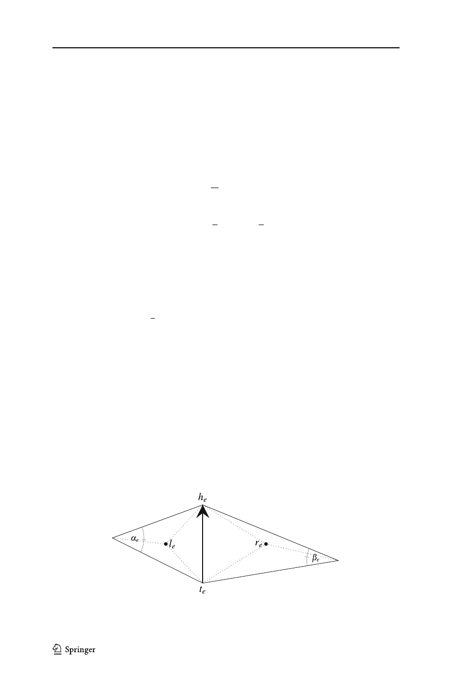
where αeand βeare the angles opposite to the edge e∈Ein the two adjacent

triangles, see Fig. 1.

(ii) If e=[x,y]is incident to a boundary triangle in Fρ,weusethechartPr

and define the weight similarly as above as a sum c(e) =C1+C2of two parts

corresponding to the two incident triangles Δ1,Δ

2. If there is a non-boundary

triangle, say Δ1,incidenttoe, we consider the angle αein this triangle opposite

to eand set C1=1

2cot αe. The second part C2=C[x,y]is defined below in (4)

using a suitable interpolation function and the smooth Dirichlet energy. More

details and explicit calculations are given in Appendix A.1.

Using our edge weights, we can define discrete harmonicity and a discrete Dirich-

let energy for functions u:V→Ron the vertices of the triangulation TR.In

particular, uis called discrete harmonic if for every vertex x∈Vthere holds



y∈V:[x,y]∈E

c([x,y])(u(y) −u(x)) =0. (2)

The energy of uis

ET(u) =

e=[x,y]∈E

c([x,y])(u(y) −u(x))2.(3)

Fig. 1 Notation associated with an edge e=[te,h

e]∈Eand with its oriented version e=−−→

tehe,see

Sections 2.1 and 2.2

23 Page 4 of 30 Math Phys Anal Geom (2021) 24: 23

The motivation for our choice of weights, in particular for the choice of weights

for boundary triangles, is the following connection of discrete and smooth Dirichlet

energies. Recall that for a continuous function on a compact Riemann surface R

which is smooth almost everywhere the Dirichlet energy is defined as

E(u) =R|∇u|2.

Then the discrete energy of a function u:V→Ris in fact the Dirichlet energy

of the continuous interpolation function ITu, defined piecewise on every triangle

Δ[x,y,z]as follows:

(i) If at least two of the three vertices x,y,z are contained in the open disc Bρ(0)

under the chart Pr

Ror in the closed disc B1/ρ(0)under the chart Pr∞

R,we

define ITu|Δ[x,y,z]on this triangle as the linear interpolation of the values of u

at the vertices.

(ii) In the remaining case, Δ[x,y,z]is a boundary triangle in Fρand under the

chart Pr

Rthere is exactly one vertex in Bρ(0),sayx. We first define ITuon the

boundary edges consistently with the definitions in (i). The two edges [x,y]and

[x,z]are straight lines. On these edges we define ITuas the linear interpolation

of the values of the vertices. On the arc 

yz connecting yand zwe use the

corresponding transformed function 

u=u◦1/z and the interpolating function

ITu|Δ[x,y,z]=

ITu

Δ◦1/z. Then for every straight line segment connecting x

to a point on the arc 

yz we define ITuas the linear interpolation of the values

on the endpoints.

Using this interpolation function, we obtain by elementary calculations (see

Appendix A.1 fordetails)that

Δ[x,y,z]|∇ITu|2=C[x,y](u(x) −u(y))2+C[y,z](u(y) −u(z))2

+C[z,x](u(z) −u(x))2,(4)

where the constants C[x,y],C

[y,z],C

[z,x]only depend on the triangle Δ[x,y,z],

see (13)–(15), and give one part of the weights associated to the edges

[x,y],[y,z],[z, x]respectively.

It is easy to see that for every triangulation of a ramified covering Rof ˆ

Cas above,

ITuis a well-defined continuous function on R. Furthermore, we have

Lemma 1 (Interpolation lemma)

E(ITu) =ET(u).

Proof We can split the energy according to triangles Δffor f∈F.

E(ITu)=

Δf⊂Bρ(0)Δf|∇ITu|2+

Δf⊂ˆ

C\Bρ(0)Δf|∇ITu|2+

Δf∈Fρ(0)Δf|∇ITu|2

In particular, elementary calculations show that (4) holds for any triangle Δ[x,y,z].

with suitable constants C[x,y],C

[y,z],C

[z,x]depending only on Δ[x,y,z]. Duffin

Page 5 of 30 23Math Phys Anal Geom (2021) 24: 23

Loading more pages...