Anticipation-induced social tipping: can the environment be stabilised by social dynamics? [original]

Eur. Phys. J. Spec. Top. (2021) 230:3189–3199

https://doi.org/10.1140/epjs/s11734-021-00011-5

THE EUROPEAN

PHYSICAL JOURNAL

SPECIAL TOPICS

Regular Article

Anticipation-induced social tipping: can the environment

be stabilised by social dynamics?

Paul Manuel M¨uller1,2,3,a, Jobst Heitzig1,J¨urgen Kurths4,5, Kathy L¨udge2, and Marc Wiedermann1

1FutureLab on Game Theory and Networks of Interacting Agents, Potsdam Institute for Climate Impact Research,

Member of the Leibniz Association, PO Box 60 12 03, 14412 Potsdam, Germany

2Institute for Theoretical Physics, Technische Universit¨at Berlin, Hardenbergstraße 36, 10623 Berlin, Germany

3Department of Neurology, Charit´e-Universit¨atsmedizin Berlin, Charit´eplatz 1, 10117 Berlin, Germany

4Department of Complexity Science, Potsdam Institute for Climate Impact Research, Member of the Leibniz Association,

PO Box 60 12 03, 14412 Potsdam, Germany

5Centre for Analysis of Complex Systems, Sechenov First Moscow State Medical University, Moscow, Russia

Received 28 November 2020 / Accepted 18 March 2021 / Published online 26 April 2021

©The Author(s) 2021

Abstract In the past decades, human activities caused global Earth system changes, e.g., climate change or

biodiversity loss. Simultaneously, these associated impacts have increased environmental awareness within

societies across the globe, thereby leading to dynamical feedbacks between the social and natural Earth

system. Contemporary modelling attempts of Earth system dynamics rarely incorporate such co-evolutions

and interactions are mostly studied unidirectionally through direct or remembered past impacts. Acknowl-

edging that societies have the additional capability for foresight, this work proposes a conceptual feedback

model of socio-ecological co-evolution with the speciﬁc construct of anticipation acting as a mediator

between the social and natural system. Our model reproduces results from previous sociological threshold

models with bistability if one assumes a static environment. Once the environment changes in response

to societal behaviour, the system instead converges towards a globally stable, but not necessarily desired,

attractor. Ultimately, we show that anticipation of future ecological states then leads to metastability of

the system where desired states can persist for a long time. We thereby demonstrate that foresight and

anticipation form an important mechanism which, once its time horizon becomes large enough, fosters

social tipping towards behaviour that can stabilise the environment and prevents potential socio-ecological

collapse.

1 Introduction

In the last decades, humanities’ impacts on the environ-

ment became increasingly more global in nature, more

rapid, extensive, and also threatening for the social and

environmental systems themselves [1–3]. Scientists refer

to this geological era as the Anthropocene due to the

impact humanity has and has had on the Earth system

[1,3]. In the Anthropocene, global challenges like cli-

mate change and resource scarcity need to be addressed

and interventions are required to build a sustainable

society which is able to overcome these challenges [4].

To improve the understanding of Earth system

dynamics in the Anthropocene, it is crucial to model

both the social and the ecological systems as coupled

together due to the interconnections and bidirectional

feedback processes between humanity and the environ-

ment [5–11], giving rise to the novel ﬁeld of World-

Earth modelling [10]. Examples of such models include

network models of individual resource use and social

ae-mail: paul-manuel.mueller@charite.de (corresponding

author)

adaptation [12,13] combined with eﬀects of governance

and taxation [14]. Other models investigate land use

and social learning [15] or land use and management

[16]. There are also models which incorporate not only

a social and ecological system but additionally include

an economic branch [17].

One important feature of the World-Earth system

is that of tipping elements. Tipping elements change

rapidly and qualitatively after surpassing a critical

threshold, the so-called tipping point [2]. In the past,

many natural tipping elements, like the Greenland-ice

sheet which can either persist or melt-oﬀ completely,

due to the melt-elevation feedback, or the Amazon,

which does either exist in today’s rainforest state or

transition into a Savannah-like state, have been identi-

ﬁed and their risk of tipping even within the 2 ◦C target

of the Paris agreement has been investigated [2,18].

On the other hand, social tipping and its poten-

tial to transform societies, so that the aforementioned

(unwanted) natural tipping may be prevented came into

research focus recently [19–22]. Social tipping can for

example be observed when a determined minority grows

larger than a critical mass and then becomes able to

123

3190 Eur. Phys. J. Spec. Top. (2021) 230:3189–3199

overturn the behaviour or conventions of the major-

ity [23,24]. Granovetter’s threshold model is an early

model formulating and explaining this phenomenon on

the example of riots [25]. For the binary decision of not

participating or participating in a riot, it is assumed

that every individual needs to observe a certain percent-

age of the population participating in the riot before

doing so themselves. This percentage is called their

(population-pertaining) threshold. From the distribu-

tion of the thresholds, one could then calculate the

equilibrium number of participants in the riot. How-

ever, real-world threshold distributions are hard to eval-

uate and reasonable guesses for the distributions lead

to everyone or no-one participating in the riot [22]. Two

possible extensions to tackle these issues are the intro-

duction of determined minorities and the explanation of

an individual’s apparent population-pertaining thresh-

old in terms of its position in the social network and

a uniform neighbour-pertaining threshold [22,26]. This

latter type of threshold determines what percentage of

a person’s acquaintances need to participate for the

person to participate itself. The wide distribution of

people’s population-pertaining thresholds then arises,

because an emerging cascade of activity reaches diﬀer-

ent locations in the network at diﬀerent stages of the

riot.

While there is already quite a consolidated under-

standing of the dynamics within single tipping ele-

ments [27,28], especially from the natural realm [29,30],

it remains an important task of ongoing research to

study interactions between diﬀerent elements, speciﬁ-

cally across the climate and the social system [9,31],

since exemplary studies have shown that such interac-

tions can give rise to substantial changes of such sys-

tems on the macro-scale [32,33]. Recent work has inves-

tigated also the interaction of tipping elements in natu-

ral [34–38], social [19], socio-economic [39], or socio-

ecological systems [40]. However, most of the afore-

mentioned studies have either studied tipping elements

using identical prototypical normal forms for each ele-

ment [35–38,40] or by focussing on cascading eﬀects and

interactions within either only natural or social subsys-

tems [19,34–38] and thus without explicitly accounting

for their potential cross-system interactions.

To bridge this gap, the present work investigates

potentially arising dynamics of coupled tipping ele-

ments across the natural and social system and pro-

poses a conceptual, low-dimensional model consisting of

a stylised environment being described by one macro-

scopic variable which we call the pollution and a social

network of individuals which change their behaviour,

i.e., either their contribution to the pollution or their

active decision to not contribute to it, according to

change probability rates based on three threshold pro-

cesses:

1. Direct environmental impacts like droughts, heat-

waves, or air pollution can threaten human society

[41–43]. An adaptation to and mitigation of these

impacts is necessary in a changing Earth system

[44].

2. Social contagion which is recognised as the spread

of behavioural patterns among many individuals in

an interacting society [45], e.g., social movements

[46–48] or the spread of social norms [49].

3. Anticipated environmental impacts are rarely dis-

cussed in World-Earth models where social system’s

are mostly coupled to the environment through

precedent or contemporary impacts. However, giv-

ing societies the capability of anticipation and fore-

sight might alter the social behavioural patterns sig-

niﬁcantly. For example, the threat of global climate

changing to the worse, like in a “Hothouse Earth”

scenario [50], could spark and strengthen climate

movements with the goal to prevent consequential

environmental impacts [51]. Especially, information

and the anticipatory time horizon up to which an

individual projects such impacts can have signiﬁ-

cant inﬂuence on the behaviour of individuals and

the macroscopic dynamics [11,52].

In particular, we incorporate the social system via

an agent-based model (ABM) similar to Ref. [22],

since ABMs have been proven as a promising tool

to model social behaviour and decision-making [53–

55]. In ABMs, individuals, called agents, adjust their

behaviour according to certain deterministic or stochas-

tic rules after assessing their individual situation [54].

One of the strengths of ABMs lies in the microscopic

details which arise from the simulation of individuals

and can induce emergent macroscopic phenomena [56].

Within ABMs, non-linear features, such as local het-

erogeneous structures, can be observed and analysed to

help understanding the impact of disturbances or causes

of unexpected outcomes [7]. However, ABMs come with

signiﬁcant computational costs and are hard to analyse

formally. Therefore, we also apply a mean-ﬁeld approx-

imation of the microscopic behaviour of the network of

interacting agents.

The model simulations presented in this work reveal

that a direct coupling between a dynamic environment

and social dynamics leads to one globally stable attrac-

tor. However, additionally accounting explicitly for the

eﬀects of anticipation induces metastability where addi-

tional environmental states that are not within or close

to that stable attractor persist over a long time.

The remainder of this paper is structured as follows.

First, in Sect. 2, the micro-level socio-ecological model

itself is introduced and the implementation of the three

aforementioned processes is explained. Second, a mean-

ﬁeld approximation of the model is given in Sect. 2.3.

Third, we give an overview of the model behaviour, ﬁrst

for a static and then a dynamic environment, and com-

pare it to the mean-ﬁeld approximation in Sect. 3.1.In

Sect. 3.2, one can ﬁnd the main results of the paper,

metastability for high anticipation times resulting in

a stabilisation of potentially unpolluted environments

and thus social tipping. We close this paper with a dis-

123

Eur. Phys. J. Spec. Top. (2021) 230:3189–3199 3191

cussion of the results, possible connections to real-world

parameters, and a breif outlook in Sect. 4.

2Model

To illustrate the inﬂuence of the environment on social

activation and vice versa, we formulate a conceptual

network model which is tuneable from a mainly social

dynamic version similar to Granovetter’s threshold

model [25]asinRef.[22] to a coupled socio-ecological

agent-based model. A focus in the model is the eﬀect of

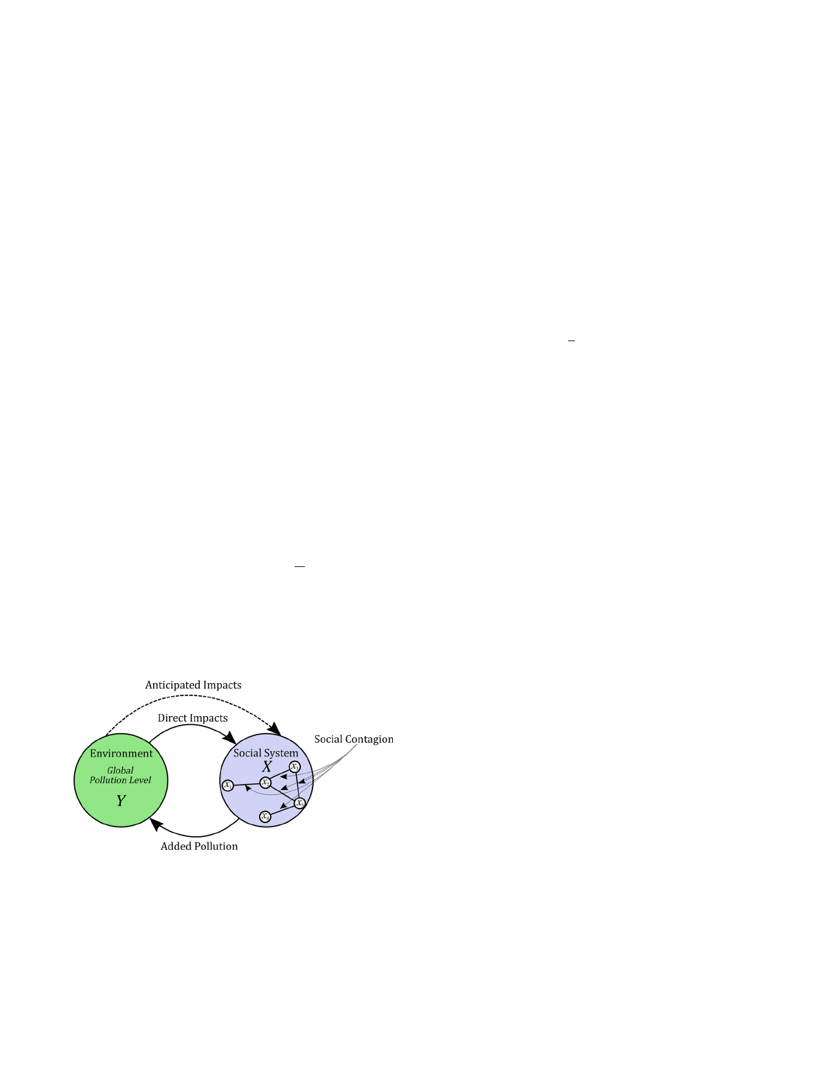
anticipation. In Fig. 1, we provide a schematic overview

of the model’s setup which illustrates the diﬀerent inter-

action mechanisms between the environment and the

social system, explained in detail below.

First, we deﬁne agent i’s pollution state as:

xi=1,for polluting (i.e., not mitigating pollution) agents

0,for non-polluting (i.e., mitigating pollution) agents .

(1)

Agents are able to switch from one state to the other,

and especially, the direction from polluting to actively

non-polluting is of importance if one wants to guide the

system towards an unpolluted state. The mean share of

polluting agents will be denoted X=1

Nixiwhere N

is the number of agents. We use this macroscopic vari-

able Xto couple the social system to the environment

which is represented by only one macroscopic variable,

the pollution Y.

Fig. 1 Schematics for the model setup. The environment is

represented by just one variable, the global pollution level

Y, which changes proportional to its own value and the

social systems mean state, the share of polluting agents

X. The social system consists of individual agents which

are either adding to the pollution or not. They change

their binary state xidepending on the current pollution

level (direct impacts), the pollution level they anticipate in

the future (anticipated impacts) and the behaviour of their

direct neighbours in the network (social contagion)

2.1 Ecological dynamics

As greenhouse gases, especially CO2, are the major

driving force of anthropogenic climate change [57,58],

we motivate our environmental module with their fun-

damental dynamics. Carbon added to the atmosphere,

for example by burning fossil fuel, does not stay in the

atmosphere, but is constantly removed through natural

carbon sinks like terrestrial ecosystems or the ocean,

with the latter being the major carbon sink in the

Earth system [59,60]. For simplicity, the carbon decay

is modelled by a linear diﬀerential equation with a sin-

gle average lifetime τ[59,61,62]. Additionally, pollution

is added proportionally to the share of polluting agents

Y=1

τ(X−Y).(2)

In particular, Yis measured in units of maximal equi-

librium pollution,sothatifallNagents pollute con-

sistently (X= 1), then Y→1. The average lifetime

of pollution, τ>0, allows to scale the system to a

quasi-static environment by letting τ→∞. Here, the

term quasi-static means that the environmental dynam-

ics become very slow in comparison to the dynamics of

the social system for which we will explain all further

details below in Sect. 2.2. However, a reasonable esti-

mate for a real-world average lifetime of atmospheric

carbon is approximately 50 years [60,61]. Consequently,

for τ= 1, one time unit in our model roughly corre-

sponds to 50 years in a real-world representation of the

Earth’s atmosphere. We are aware that this implemen-

tation of the environment is very conceptual and that

there are also comparatively more advanced models of

the carbon cycle [59,63–65]. However, for the qualita-

tive behaviour of our model only some form of natural

decay is necessary, so the environmental dynamics from

Eq. (2) suﬃces.

2.2 Social dynamics

The social dynamics of the share of polluting agents

Xarise from the dynamics of the single agents’ states

x=(xi)N

i=1. The agents change their states with the

change probability rates p−

i(x,Y) from polluting to

non-polluting (xi=1→xi=0)andp+

i(x,Y)from

non-polluting to polluting (xi=0→xi= 1):

p−

i(x,Y)=α·p−

dir(Y)+β·p−

i,soc(x)·p−

ant(X,Y ),

(3)

i(x,Y)=α·p+

dir(Y)+β·p+

i,soc(x)·p+

ant(X,Y ).

(4)

There are three contributions to the change probability

rates which we will motivate and explain in detail in the

following paragraphs: those due to direct environmental

impacts, p±

dir(Y), due to social contagion, p±

i,soc(x), and

due to anticipated environmental impacts, p±

ant(X,Y ).

123

3192 Eur. Phys. J. Spec. Top. (2021) 230:3189–3199

The ﬁrst contribution is scaled by a parameter α≥0

which we call the vulnerability, since one could interpret

it as how susceptible an agent is to immediate changes

in their environment. The second and third contribu-

tions are coupled together and are scaled by a param-

eter β≥0 which we call the farsightedness, since it

weights the anticipation eﬀect. This coupling can be

understood as social contagion leading to a spread of

the action due to anticipated environmental impacts.

Note that among these factors, only p±

i,soc(x) depends

on the microstate x, while the others only depend on

the macrostate (X,Y ).

2.2.1 Direct environmental impacts

Direct environmental impacts like droughts or storms

have triggered sudden societal changes in the past,

including the onset of migratory patterns or even the

collapse of whole nations [66,67]. In our model, we link

the behaviour of agents to the current pollution level Y

through a threshold function. If the pollution is above

the pollution threshold parameter γ∈[0,1], a polluting

agent has a higher probability to become non-polluting

and vice versa:

p−

dir(Y)=H(Y−γ),(5)

dir(Y)=1−H(Y−γ),(6)

where His the Heaviside step function.

2.2.2 Social contagion

The embedding of individuals in a social network and

the observation of their immediate surroundings has

been proven to have a large inﬂuence on people’s

behaviour [45,49,68,69]. Recently proposed network

models allow to incorporate and explain such dynam-

ics in the context of opinion formation [70], behaviour

[68,71] and information spread [72] or social move-

ments and collective action [69]. Granovetter’s thresh-

old model [25] and recent network-based extensions

[22,73–75] describe such inﬂuence by other individ-

uals or direct neighbours, also known as social con-

tagion [76]. From Refs. [22,26], we take the idea to

deﬁne a microscopic neighbour-pertaining threshold χ∈

[0,1] which inﬂuences the likelihood of the agents’

behavioural change. If the share of polluting neigh-

bours in the ﬁxed social network G,Xi

ki, is lower than

the social threshold χ, a polluting agent becomes more

likely to convert to being non-polluting and vice versa.

Here, Xi=|{j:(i, j)∈E, xj=1}| gives the number

of polluting neighbours, ki=|{j:(i, j)∈E}| is i’s

degree (number of neighbours), and Eis the ﬁxed set

of network edges:

p−

i,soc(x)=1−HXi

−χ,(7)

i,soc(x)=HXi

−χ.(8)

2.2.3 Anticipated environmental impacts

The anticipation of potential environmental catastro-

phes might spark, strengthen, and justify climate move-

ments like the recent Fridays for Future-movement [51].

Speciﬁcally, the anticipation time, i.e., how far one

extrapolates the trajectory of the Earth system into the

future, can have a big impact on the social urge to act

[11,52]. We assume the simplest possible form of antic-

ipation, a linear extrapolation, and therefore deﬁne the

anticipated pollution as:

Yant =Y+θ˙

Y, (9)

where θ>0istheanticipation time. If the anticipated

pollution is above the pollution threshold γ, a polluting

agent becomes more likely to get non-polluting. Like-

wise, if it is below, a non-polluting agent becomes more

likely to get polluting:

p−

ant(X,Y )=HY+θ˙

Y−γ

=HY+θ

τ(X−Y)−γ,(10)

ant(X,Y )=1−HY+θ˙

Y−γ

=1−HY+θ

τ(X−Y)−γ.(11)

Plugging these factors into Eqs. (3,4) yields the full

change probability rates:

p−

i(x,Y)=αH(Y−γ)+β[1 −H(Xi−χki)]

×HY+θ

τ(X−Y)−γ,(12)

i(x,Y)=α[1 −H(Y−γ)] + βH(Xi−χki)

×1−HY+θ

τ(X−Y)−γ,

(13)

which together with Eq. (2) fully deﬁne our system for

a given network structure.

2.3 Mean-field approximation

Applying a mean-ﬁeld approximation and therefore

eliminating the explicit network dependence allows us

to get important insights into the systems dominant

dynamics. We therefore assume that the network is

large, densely connected, and has a small diameter, such

that changes spread fast through the network and thus,

most of the time, the share of polluting neighbours is

approximately equal for all nodes. Consequently, the

latter can be approximated well by the overall share of

polluting agents:

≈X. (14)

123

Eur. Phys. J. Spec. Top. (2021) 230:3189–3199 3193

Plugging this into Eqs. (7,8) cancels out the network

dependence and all agents have approximately the same

change probability rates:

p−(x,Y)≈˜p−(X, Y )=αH(Y−γ)+β[1−H(X−χ)]

×HY+θ˙

Y−γ,(15)

p+(x,Y)≈˜p+(X, Y )=α[1−H(Y−γ)]+βH(X−χ)

×1−HY+θ˙

Y−γ.(16)

Since the network is also assumed to be very large, the

actual stochastic change in Xcan be approximated by

its expectation value and we obtain ﬁnally the deter-

ministic diﬀerential equations:

X=(1−X)˜p+(X,Y )−X˜p−(X,Y ),

Y=1

τ(X−Y).(17)

Through this approximation, we reduced the num-

ber of equations from 2N+ 1 to only two (however

non-smooth) diﬀerential equations which can be solved

numerically. In addition, a piece-wise analytical solu-

tion is possible, since the change rates p±are constant

except when Xhits the threshold χor when Yor

Yant hits the threshold γ. For constant p±, the diﬀer-

ential equations become linear in Xand Yand can be

solved through an exponential ansatz and the method

of varying constants (see S1). However, due to the non-

smoothness, it is not possible to ﬁnd a full solution,

but only such a piece-wise solution. For the numeri-

cal implementation, we used the piece-wise calculated

equations for Xand Yand probed through integrat-

ing for discrete time steps which particular piece-wise

solution has to be used each time t.1

3Results

In the ﬁrst part of this section, we compare the dynam-

ics of the microscopic model to the dynamics of the

above introduced mean-ﬁeld approximation. First, the

case of a static environment is studied, i.e., the social

dynamics are signiﬁcantly faster than the environmen-

tal dynamics (α,β =const.,τ→∞), to show that our

model displays a bistable behaviour as also found in

other works on social tipping [22,74]. Second, we study

the case of a dynamic environment, i.e., the social sys-

tem evolves on a similar timescale as the environmen-

tal system, and we investigate the attractors of this

feedback system. Subsequently, we use the mean-ﬁeld

approximation and identify multi-stability in the regime

of long anticipation times.

1Implementations of the mean-ﬁeld model and the agent-

based simulations are available online at https://github.

com/PaulMMueller/GranoEnv.

3.1 Comparing the microscopic model to the

mean-field approximation

We compare the mean-ﬁeld approximation with micro-

scopic model simulations for Erd˝os–R´enyi networks

with N= 200 nodes and an average degree of ¯

k= 10.

Calculations are robust against larger network size, so

that ﬁnite-size eﬀects are negligible in the presented

results (not shown). In Fig. 2a–d, results for a static

environment (τ=10

6) are displayed. Additionally, the

social system does not directly respond to the envi-

ronment (α= 0) but only to the anticipated impacts

(β= 10). These parameter choices ensure that the

dynamics are dominantly driven by social contagion, see

Eqs. (3,4), so that we can compare our model in this

boundary case against other studies [22,74]. The micro-

scopic results are shown in Fig. 2a, b and the mean-

ﬁeld approximation results in Fig. 2c, d. In Fig. 2a,

c, the distribution of the long-term share of polluters,

p(X(t= 20)), is shown as a histogram. In both cases,

we observe two prominent maxima at X=0andX=1

which compares well to previous network-based thresh-

old models that are showing bistability, as well [22,74].

The exemplary trajectories in Fig. 2b, d show that the

trajectories approach X=0ifY⩾γand X<χ.In

the microscopic case, Fig. 2b, trajectories with X(t=0)

slightly above χcan approach the attractor at X=0,

even though the social system would be above the social

threshold. This can be explained through the local het-

erogeneity of the network leading to some nodes in an

environment with Xi

ki<χ, even though X⩾χ. These

nodes can then start a cascade eventually leading to

all nodes approaching the same state. In the mean-

ﬁeld approximation, Fig. 2d, such a behaviour cannot

be observed as X<χand Y+θ˙

Y⩾γresults in

all change rates becoming zero. To account for these

mismatches, future work should explore more advanced

approximation techniques, such as heterogeneous mean-

ﬁeld approximations [77] to provide a better represen-

tation of the model’s dynamics for those limiting cases

as well. Since most other trajectories and the distribu-

tions of steady states, however, match well across the

numerical experiments and the analytical estimations

we consider our approximation to perform suﬃciently

well for the purpose of the present study.

In Fig. 2e–h, we introduce a dynamic environment

(τ= 1) and couple the social system directly to the

environment (α=0.1). The system again reaches its

attractor before t= 20, and in Fig. 2e, g, the distribu-

tion of X(t= 20) is displayed. In contrast to the static

environment case, it peaks around X≈Y≈γfor both

the microscopic simulations (Fig. 2e) and the mean-ﬁeld

calculations (Fig. 2g). The existence of only one main

attractor around X≈Y≈γis emphasized through the

trajectories in Fig. 2f, h which in the long-term show

the same behaviour for microscopic and mean-ﬁeld sim-

ulations. However, in the transient phase (t<2), the

microscopic simulations still diﬀer from the mean-ﬁeld

solution due to the heterogeneity of the underlying net-

work. The coupling to a dynamic environment, Fig. 2e–

123

Loading more pages...