Study on the transition behavior of the bulging effect during deep penetration laser beam welding [original]

International Journal of Heat and Mass Transfer 184 (2022) 122171

Contents lists available at ScienceDirect

International Journal of Heat and Mass Transfer

journal homepage: www.elsevier.com/locate/hmt

Study on the transition behavior of the bulging effect during deep

penetration laser beam welding

Antoni Artinov

a , ∗, Xiangmeng Meng

, Marcel Bachmann

, Michael Rethmeier

b , a , c

Bundesanstalt für Materialforschung und prüfung (BAM), Unter den Eichen 87, 12205 Berlin, Germany

Institute of Machine Tools and Factory Management, Technische Universität Berlin, Pascalstrae 8-9, 10587 Berlin, Germany

Fraunhofer Institute for Production Systems and Design Technology, Pascalstrae 8-9, 10587 Berlin, Germany

a r t i c l e i n f o

Article history:

Received 5 July 2021

Revised 5 October 2021

Accepted 22 October 2021

Available online 9 December 2021

Keywords:

Laser beam welding

Deep penetration

Bulge formation

Numerical modeling

a b s t r a c t

The present work is devoted to the study of the transition behavior of the recently conﬁrmed widening

of the weld pool, known as the bulging effect, during high-power deep penetration laser beam welding of

thick unalloyed steel sheets. A three-dimensional transient multi-physics numerical model is developed,

allowing for the prediction of the bulge formation and the study of its temporal behavior. The model

is generalized to account automatically for the transition from partial to complete penetration. Several

experimental measurements and observations, such as drilling period, weld pool length, temperature,

eﬃciency, and metallographic cross-sections are used to verify the model and assure the plausibility of

the numerical results. The analysis of the calculated temperature and velocity distributions, as well as the

evolution of the keyhole geometry, shows that the formation of a bulging region strongly depends on the

penetration depth of the weld. Based on the numerical results, the bulge is found to occur transiently,

having its transition from a slight bulge to a fully developed bulging between penetration depths of 6 mm

and 9 mm, respectively.

This is an open access article under the CC BY-NC-ND license

( http://creativecommons.org/licenses/by-nc-nd/4.0/ )

1. Introduction

In the last decade the development of modern laser systems

with high-power of up to 100 kW for solid state lasers enabled

joining sheets with a thickness of up to 50 mm by a single pass

welding [1–3] . Nowadays, the laser beam welding process brings

several technical advantages compared to conventional arc welding

processes, such as low distortion of the welded components due to

the locally highly concentrated and precise heat input, high reach-

able welding speed, narrow heat affected zone, etc. [4] . Hence,

the application of the laser beam welding process on sheets of

higher thickness offers a great potential for more effective join-

ing, e.g., by the production of high pressure and vacuum vessels,

crane construction, as well as in the shipbuilding and aerospace

industry.

However, with the increase of welding speed and sheet thick-

ness, new challenges arise, such as untypical defect formation for

speciﬁc materials, e.g., hot-cracking during welding of unalloyed

∗Corresponding author.

E-mail address: [email protected] (A. Artinov).

and low-alloyed steel sheets [5–7] . Although, hot-cracking is one

of the most studied material phenomena from the welding ﬁeld,

its nature remains highly complex [8,9] . Nevertheless, it is a well-

known fact that the interaction between the three crucial factors,

namely the thermal, mechanical, and metallurgical factor, is deci-

sive for the cracking susceptibility of the welded specimen [10] .

Hereby, their interaction is strongly dependent on the weld pool

shape and vice versa, see, e.g., [11] . The importance of this de-

pendency was demonstrated back in the early 1980s during stud-

ies on deep penetration electron beam welding. In these studies,

a geometric particularity, or more precisely a local disturbance of

the solidiﬁcation front was observed in the longitudinal section of

the welded specimen by adding a pure Ni-wire at different po-

sitions along the thickness of the specimen. The disturbance led

to a local delay in the solidiﬁcation behavior, which led to an in-

crease in the cracking sensitivity of the welded component [12–

15] . To the best of the author’s knowledge, there are only a few re-

search results published on the occurrence of the widening of the

weld pool interface during welding with high power lasers, nowa-

days referred to as the bulging effect. In more recent studies, so-

phisticated modern visualization techniques combining transparent

https://doi.org/10.1016/j.ijheatmasstransfer.2021.122171

( http://creativecommons.org/licenses/by-nc-nd/4.0/ )

A. Artinov, X. Meng, M. Bachmann et al. International Journal of Heat and Mass Transfer 184 (2022) 122171

Table 1

Standardized and measured chemical composition of the materials used in wt%.

Material C Si Mn P S Cu Fe

EH36-N 0.132 0.26 1.4 - - 0.012 bal.

S355J2 + N 0.088 0.34 1.38 - - 0.028 bal.

DIN EN 10025 ≤0.2 ≤0.55 ≤1.6 ≤0.025 ≤0.035 ≤0.55 bal.

quartz glass with high speed imaging and thermal camera record-

ing have been utilized to overcome the limited experimental ac-

cessibility and capture the transient behavior of the bulging effect

[11,16] . Furthermore, attempts to quantify the bulge during hybrid

laser-gas metal arc welding by deﬁning an angle determined from

the narrowest and widest cross-sectional dimensions within the

bulging region has been made in [17,18] . Although the latest re-

search proves the existence of the bulging effect during laser beam

welding of thick sheets, the obtained data does not allow for a

complete investigation or quantiﬁcation of the weld pool widen-

ing, e.g., the study of its formation mechanisms or its inﬂuence on

crucial factors for the formation of defects.

In the present time, due to the rising computational perfor-

mance, numerical simulations have brought signiﬁcant insights

into the investigation of complex phenomena. Even though not

being the object of investigation, the bulging effect can be found

in several numerical works, see, e.g., [19–25] . Its inﬂuence on the

mechanical factor, or more precisely on the temporal strain/stress

evolution in the critical bulging region, has been studied in [7,26] .

Further development on this study has been achieved by mak-

ing use of the equivalent heat source (EHS) technique proposed

ﬁrst in [27] , see, e.g., [28,29] . The EHS approach enables the pre-

cise coupling of the weld pool shape predicted with a thermo-

ﬂuid dynamics simulation and the subsequent thermo-mechanical

computation [30,31] . An overview of the relationship between the

bulging effect and the hot cracking formation during deep pen-

etration laser beam welding, where all three critical factors are

considered, can be found in the author’s previous study, see [32] .

In their study, the authors emphasize on the interaction between

the bulge and the extended solidiﬁcation temperature range due

to the accumulation of elements constituting low melting eutec-

tic, such as sulfur and phosphorous, and their segregation. As

described above and in [33,34] , such solidiﬁcation delay has al-

ready been found to decrease the cracking resistivity of the welded

component.

Based on the literature review it can be concluded that the

bulging effect plays a crucial role in the formation of defects

during deep penetration laser beam welding. Yet, the majority

of numerical works published on this topic either do not study

the bulging phenomenon at all or rather concentrate on its phe-

nomenological reproduction to estimate its inﬂuence on critical

factors, such as the three main factors determining the cracking

susceptibility of the specimen mentioned above. Hence, further nu-

merical analysis of this phenomenon is essential for the under-

standing of the laser process and the setting of the relevant process

parameters.

The present study seeks to deepen the level of understanding

by emphasizing on the formation of the bulge and more speciﬁ-

cally on its correlation to the penetration depth of the weld. Thus,

an effort is made to develop a three-dimensional transient multi-

physics numerical model taking into account the most impor-

tant physical phenomena, such as dynamic keyhole evolution, en-

ergy absorption by laser reﬂections, vaporization, thermo-capillary,

and natural convection, latent heat of phase transformations, and

temperature-dependent material properties. Furthermore, an ex-

tensive amount of experimental data is measured to fully verify

the predictions made by the model.

Table 2

Process parameters of the experiments.

Parameters Value

Wave length 1030 nm

Fibre diameter 200

μm

Beam parameter product (BPP) 8 mm mrad

Optical system HIGHYAG BIMO HP

Focal diameter 500

μm

Focal length 300 mm

Rayleigh length 6.9 mm

Material EH36-N S355J2 + N

Penetration partial complete partial

Sheet thickness 8 mm 8 mm 12 mm

Laser power 5 kW 8 kW 8 kW

Focal position 0 mm

Welding speed 2 m min

−1

Laser torch angle 0

◦

Shielding gas nozzle angle 35

◦

Shielding gas Ar, 25 l min

−1

2. Materials and Methods

2.1. Materials

Two kinds of unalloyed steel sheets with different thicknesses

were utilized in the welding experiments; a 8 mm thick high

strength steel for ship structures EH36-N and a 12 mm thick struc-

tural steel S355J2+N. The dimensions of the EH36-N and S355J2+N

sheets were 300 mm x 100 mm x 8 mm and 175 mm x 100 mm

x 12 mm, respectively. The corresponding chemical compositions

were measured with spectral analysis and are given in Table 1 .

2.2. Experiments

A 16 kW disc laser Trumpf 16002, a diode laser illumination,

and a FASTCAM SA4 high speed camera from Photron were utilized

in the experiments. Note that the experiments have been especially

designed to obtain a suﬃcient amount of data for the calibration

of the model and the validation of the numerically obtained weld

pool geometries and ﬂuid ﬂow patter therein, which determine the

formation and the dimensions of the bulging region. All welds pro-

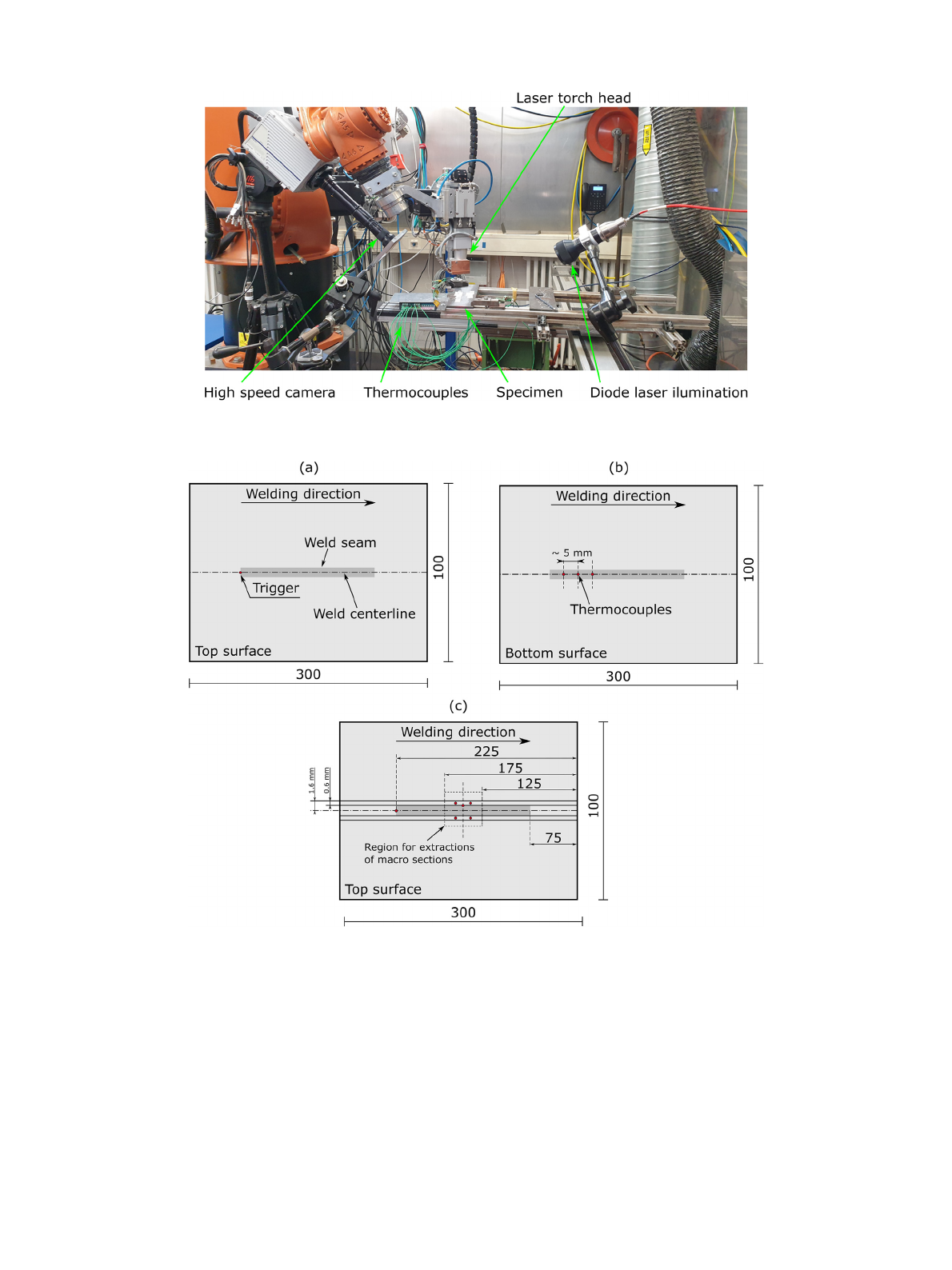
duced in the experiments were bead-on-plate welds. A schema of

the experimental setup is shown in Fig. 1 ; the process parameters

are summarized in Table 2 .

The high speed camera was set at 10 0 0 frames per second and

the laser power of the diode laser to 200 W. Altogether the exper-

iments have been divided into three parts. First, an estimation of

the drilling time for the complete penetration welding process on

8 mm thick EH36-N sheets has been obtained. For this measure-

ment, the lens optical axis of the high speed camera was placed

to be perpendicular to the longitudinal section of the sheet. Thus,

allowing to capture the very ﬁrst laser reﬂection on the top sur-

face and the moment when the laser light goes through the com-

pletely penetrated keyhole on the bottom surface. Thermocouples

were positioned along the weld centerline as shown in Fig. 2 a).

Thereby, one thermocouple was placed on the top surface of the

specimen to trigger the measurement and three further thermo-

A. Artinov, X. Meng, M. Bachmann et al. International Journal of Heat and Mass Transfer 184 (2022) 122171

Fig. 1. Schema of the experimental setup.

Fig. 2. Position of the thermocouples for the measurement of the: (a)-(b) laser drilling time and (c) time-temperature curves.

couples with a distance of approximately 5 mm were placed on the

bottom surface to measure the time temperature curves. According

to the measured curves the moment of reaching complete pene-

tration has been estimated. This part of the experiment was re-

peated three times to get an accurate averaged value of the drilling

period.

In the second part of the experiment, the partial penetration

welds on the same specimens were performed. During welding,

the weld pool length on the top surface was recorded by the high

speed camera and the thermal history at several locations was

measured by thermocouples, see Fig. 2 b). The thermocouples used

in the investigation were of type K with a diameter of 0.25 mm.

Their exact positions were measured after the welding process

with an optical microscope. It is worth noting that preliminary ex-

periments have been performed to estimate the region where the

thermocouples should be placed as well as to get an estimation

about the thickness above which the bulging effect becomes visi-

ble. In the last part of the experiments the 12 mm thick S355J2+N

sheets were welded without additional measurements. Macro sec-

tions have been extracted from the region marked in Fig. 2 c) for

the sheets welded in the second and third part of the experiments.

From these, several metallographic cross-sections have been pre-

pared with a 2% nital etching, which subsequently have been com-

pared to the numerical results.

A. Artinov, X. Meng, M. Bachmann et al. International Journal of Heat and Mass Transfer 184 (2022) 122171

2.3. Numerical modelling

A three-dimensional thermo-ﬂuid dynamics model accounting

for the free surface tracking by the volume of ﬂuid (VOF) approach

has been developed for the prediction of the bulge formation. The

model is based on several previous works with some further im-

provements and adaptions. More details can be obtained from [35–

39] .

2.3.1. Assumptions

Although, in modern time the computational capacity has been

allowing for the numerical analysis of more complex tasks, still se-

vere simpliﬁcations need to be made in order to obtain a solution

in a feasible computational time. Another reason for the simpli-

ﬁcations made in the model is the complex physics behind the

laser beam welding process including a number of strongly cou-

pled, highly-nonlinear interactions between the laser radiation, the

vapor phase, the molten metal, and the solid material. The main

assumptions made in the simulation are summarized as follows:

• The molten metal is assumed to be Newtonian and incompress-

ible, whereby the ﬂow regime of the liquid metal is considered

to be laminar.

• The ﬂow regime of the vapor phase in the keyhole is assumed

to be laminar.

• The Boussinesq approximation is used to model the impact of

the density deviation caused by the temperature difference on

the ﬂow.

2.3.2. Governing equations

The governing equations describing the multi-physics model in

a ﬁxed Cartesian coordinate system are given below. The VOF tech-

nique is employed to track the transient deformation of the molten

pool free surface and solidiﬁed weld seam proﬁle.

• Volume fraction conservation

∂ αv ol

steel

∂t + ∇ ·

v αv ol

steel

= 0 , (1)

where αv ol

steel

denotes the volume fraction of the steel phase in

a control volume and



v = (v

, v

) is the ﬂuid velocity vector.

There are three possible conditions for the control volume deﬁned

by the volume fraction of the steel, namely a control volume con-

taining only the air phase, αv ol

steel = 0 , a control volume contain-

ing only the steel phase, αv ol

steel = 1 , and a mixture control vol-

ume containing the interface between the steel and the air phases,

0 < αv ol

steel

< 1 . Note that the volume fraction conservation equa-

tion is solved only for the steel phase; the volume fraction of the

air phase is computed based on the following constraint:



i =1

αv ol

= 1 , (2)

where the subscript, i = 1 , denotes the steel phase and, i = 2 ,

the air phase [40] . The steel-air interface is reconstructed using a

piecewise-linear approach, assuming that the interface has a lin-

ear slope within each control volume [41] . The free surface of the

molten pool and the solidiﬁed weld is approximated with volume

fraction values between 0.2 and 1 and empirically determined crit-

ical volume fraction gradient value.

• Mass conservation

∇ ·

v = 0 . (3)

Note that the density is not appearing in the equation due to

the assumptions made above.

• Momentum conservation

A single momentum equation is solved throughout the compu-

tational domain. Thus, the resulting velocity ﬁeld is shared among

the phases and the material properties in each cell are averaged by

the volume fraction, e.g., the density is calculated as follows:

ρmix

= αv ol

steel

ρsteel

1 −αv ol

steel

ρair

, (4)

where ρmix

is the volume-fraction-averaged density; ρair

and ρsteel

are the densities of the air and steel phases, respectively. All other

properties except the thermal expansion coeﬃcient, for example,

the viscosity or thermal conductivity, are computed in this manner.

Thus, the momentum equation reads:

ρmix

∂



∂t +

(



v ·∇

)



= −∇ p + μmix

∇



v + ρmix



g +



, (5)

where tis the time, pis the ﬂuid pressure, μmix

is the dynamic

viscosity,



g is the gravitational acceleration vector, and



m is the

source term. The source term is deﬁned as follows:



m = −ρsteel



g βsteel

T −T

liq

+

1 −αliq

2

α3

liq

+ A

mush



sur f.tension



rec



v apor

, (6)

where βsteel

is the thermal expansion coeﬃcient, T is the tempera-

ture, T

liq

is the liquidus temperature of the unalloyed steel taken as

the reference temperature here, αliq

is the liquid volume fraction,

is a small number ( 1 ×10

−3

) use d to avoid division by zero, and

mush

is the mushy zone constant.

The ﬁrst term on the right hand side (RHS) describes the

thermal buoyancy due to the variations of the density of the

steel with temperature [42] . The second term on the RHS de-

scribes the deceleration of the ﬂow in the mushy zone which

is related to the inverse of the size of the interdendritic struc-

ture. Thereby, the mushy zone constant A

mush

is a measure

for the amplitude of the damping, thus it should be very

large ( in the current study the value is ∼5 ×10

kg m

−3

−1

) to al-

low for a steeper transition of the velocity of the material to zero

as it solidiﬁes [43,44] . The liquid fraction αliq

reads:

αliq

⎧

⎨

⎩

0 for T ≤T

sol

T −T

sol

liq

−T

sol

for T

sol

< T < T

liq

1 for T ≥T

liq

(7)

where T

sol

denotes the solidus temperature of the material used.

Additionally, the effective viscosity approach is used to model the

ﬂow in the mushy zone. Therefore, the mushy zone is divided

into three subregions depending on the coherent solid fraction

= 0 . 48 and the critical solid fraction F

= 0 . 64 . Note that the

drag coeﬃcient and the local viscosity differ in each region. The

local effective viscosity is expressed as a function of the solid frac-

tions [45] :

μsteel

= μ0

1 −F

−1 . 55

, for F

 = F

, (8)

where μ0 is the dynamic viscosity at T

liq

and F

s is the solid frac-

tion. Note that the local viscosity value in control volumes with a

solid fraction higher than the critical solid fraction was set to 200

Pas. The third term in Eq. 6 includes the effects of surface tension

along the steel-air interface. Thereby, the tangential stress terms,

also known as the Marangoni stress, arising due to the variation of

the surface tension are expressed as:

τMa

∂γ

∂T

∂



, (9)

A. Artinov, X. Meng, M. Bachmann et al. International Journal of Heat and Mass Transfer 184 (2022) 122171

where γis the surface tension and



t is the surface unit tangential

vector. The surface tension is expressed as [46] :

γ= γ0

−ˆ

T −T

liq

−R

T s

(

1 + K

)

with K

= k

exp

−H

T ,

(10)

where γ0 is the surface tension of the pure metal (in the present

study this is iron),

A is the negative slope of γas function of the

temperature, R

g is the universal gas constant, s is the surface ex-

cess at saturation, a

is the thermodynamic activity, k

is a constant

related to the entropy of segregation, and H

is the standard heat

of adsorption. Note that the value for the thermodynamic activity

was taken as the maximum allowed value according to the stan-

dard given in Table 1 . The pressure difference along the steel-air

interface, known as the Laplace pressure or the capillary pressure

is given as:

= γκ, (11)

with κ= ∇ ·



n deﬁned as the curvature in terms of the divergence

of the surface unit normal vector,



n =



n |

;



n = ∇αv ol

steel

is the in-

ward surface normal vector deﬁned as the gradient of the volume

fraction of the steel phase. The forces acting on the steel-air inter-

face are expressed as volume forces using the divergence theorem

according to the continuum surface force (CSF) model [47] . There-

fore, a transformation term is deﬁned as follows:

CSF

momentum

ρmix

|∇αv ol

steel

(

ρair

+ ρsteel

)

, (12)

allowing to compute the volume force as:



surf.tension

(

CSF

momentum

)



n . (13)

The fourth term in Eq. 6 describes one of the main driving forces

on the keyhole surface, namely the evaporation-induced recoil

pressure. The recoil pressure is calculated according to [48] and

transferred to a volume force as follows:

rec

√

exp

−M

mol

T ,



rec

(

rec

CSF

momentum

)



n , (14)

where A is numerical coeﬃcient depending on the ambient pres-

sure and its value is approximately 0 . 55

√

K for practical appli-

cations; B

0 is a vaporization constant, which in the case of iron

equals 3 . 9 ×10

2 kg m

−1

−2

; M

mol

is the molar mass, and h

v is

the latent heat of vaporization. The ﬁfth term on the RHS of

Eq. 6 includes empirical formulations of the vapor-induced stag-

nation pressure p

v apor and shear stress τv apor

, based on the as-

sumption of a laminar ﬂow within the keyhole [49] . According to

[19] these read:

v apor

= p

ρv apor



, (15)

τv apor

fρv apor



, (16)

where p

is the vapor or atmospheric pressure, ρv apor is the metal-

lic vapor density calculated with the ideal gas equation,



and



are the normal and tangential projections of the vapor veloc-

ity vector,



V , on the steel-air interface, respectively, and f = 64 / Re .

In the present work, the metallic vapor velocity vector acts verti-

cally in thickness direction and is assumed to have a magnitude

of 150 ms

−1 at the keyhole entrance [50] . Furthermore, the vapor

velocity is deﬁned as a function of the penetration/keyhole depth,

depth

, increasing linearly from 0 ms

−1 at the keyhole bottom to

its maximum value at the keyhole entrance in the partial pene-

tration case. Note that in the complete penetration case, there are

two metallic vapor velocity vectors acting in opposite directions. In

this case, one vector increases linearly, starting at two-thirds of the

plate thickness, reaching 150 ms

−1 at the keyhole entrance and a

second vector increasing in the same manner towards the keyhole

exit, reaching 100 ms

−1

at the sheet bottom [51,52] . The projection

of the vapor velocity vector onto the surface unit normal vector,



n ,

of the steel-air interface can be calculated as follows:





V ·





n . (17)

The tangential projection of the vapor velocity can then be calcu-

lated by the following vector equation:



V −



. (18)

Equation 16 is further simpliﬁed by substituting the Re number

and finto it:

τv apor

8 μT

max



, (19)

where D is the averaged diameter of the keyhole and μT

max

is the

dynamic viscosity at the maximum reachable temperature set in

the model. For the calculation of D , the keyhole volume, V

key

, is

approximated as a cylindrical pipe with the length of the keyhole

depth, h

depth

, leading to:

D =



4 V

key

depth

π. (20)

The dynamic viscosity at T

max is approximated by the kinematic

theory of gases as follows:

μT

max

mol

√

2 ˆ σ

8 k

max

πM

mol

, (21)

where ˆ σ= πd

mol

is the collision cross-section of the molecule

with d

mol

the molecular diameter and k

is the Boltzmann con-

stant. In the particular case of the unalloyed steel utilized in this

study, see Table 1 , the value of the dynamic viscosity is approx-

imately 1 . 62 ×10

−4

kg m

−1

−1 for a super-heating temperature of

3400 K [53,54] . Finally, the corresponding source term can be given

as follows:



v apor



stagnation



shear

with



stagnation

(

v apor

CSF

momentum

)



n ,

and



shear

(

τv apor

CSF

momentum

)



t .

(22)

The CSF method is applied here for the transformation of the stag-

nation pressure and the shear stress to volume forces according to

[55] .

• Energy conservation

ρmix

∂ H

mix

∂t +

(



v ·∇

)

mix

= ∇ ·(

λmix

∇T

)

+ S

, (23)

where H

mix

is the enthalpy, λmix

is the heat conductivity, and S

e is

the source term. The enthalpy of the material is computed as the

sum of the sensible enthalpy, h

mix

, and the latent heat of fusion of

the material used, h

, as follows:

mix

= h

mix

+ h

, (24)

with h

mix

given as:

mix

= h

ref

 T

ref

mix

dT . (25)

Here, the subscript, re f, stands for reference, thus h

ref

is the refer-

ence enthalpy and T

ref

is the reference temperature; c

mix

is the

speciﬁc heat at constant pressure. Furthermore, the latent heat

content, L , in each control volume, is written in terms of the la-

Loading more pages...