Correcting surface loading at the observation level: impact on global GNSS and VLBI station networks [original]

Journal of Geodesy manuscript No.

(will be inserted by the editor)

Correcting surface loading at the observation level: Impact on

global GNSS and VLBI station networks

Benjamin M¨annel ·Henryk Dobslaw ·Robert Dill ·Susanne Glaser ·

Kyriakos Balidakis ·Maik Thomas ·Harald Schuh

Received: date / Accepted: date

Abstract

Time-dependent mass variations of the near-

surface geophysical fluids in atmosphere, oceans and the

continental hydrosphere lead to systematic and signif-

icant load-induced deformations of the Earth’s crust.

The Earth System Modelling group of Deutsches Geo-

ForschungsZentrum (ESMGFZ) provides vertical and

horizontal surface deformations based on numerical mod-

els of the global geophysical fluids in atmosphere, oceans

and the continental hydrosphere with a spatial resolution

of 0.5

◦

and a temporal sampling of down to three hours

(Dill and Dobslaw, 2013). The assessment of conven-

tionally – i.e. without consideration of non-tidal loading

models – processed global GNSS datasets reveals that

large parts of the residual station coordinates are indeed

related to surface loading effects. Residuals explained by

the models often have a pronounced annual component,

but variability at other periodicities also contributes to

generally high correlations for seven-day averages. More

than ten years of observations from about 400 GNSS

and 33 VLBI stations were specifically reprocessed for

this study to incorporate non-tidal loading correction

models at the observation level. Comparisons with the

corresponding conventional processing schemes indicate

that the coordinate repeatabilities and residual annual

B. M¨annel

H. Dobslaw

R. Dill

S. Glaser

K. Balidakis

M. Thomas ·H. Schuh

Deutsches GeoForschungsZentrum GFZ, Telegrafenberg,

14473 Potsdam, Germany

E-mail: benjamin.maennel@gfz-potsdam.de

M. Thomas

Institute of Meteorology, Freie Universit¨at Berlin, Carl-

Heinrich-Becker-Weg 6-10, 12165 Berlin, Germany

H. Schuh

Institute of Geodesy and Geoinformation Science, Technische

Universit¨at Berlin, Strasse des 17. Juni 135, 10623 Berlin,

Germany

amplitudes decrease by up to 13 mm and 7 mm, respec-

tively, when ESMGFZ’s loading models are applied. In

addition, the standard deviation of the daily estimated

vertical coordinate is reduced by up to 6.8 mm. The

network solutions also allow for an assessment of surface

loading effects on GNSS satellite orbits, resulting in

radial translations of up to 4 mm and Earth orientation

parameters (EOP). In particular the VLBI-based EOP

estimates are critically susceptible to surface loading

effects, with root-mean-squared differences reaching of

up to 0.2 mas for polar motion, and 10

s for UT1-UTC.

Keywords

GNSS

VLBI

non-tidal surface loading

GNSS orbits ·polar motion

1 Introduction

The redistribution of mass within the interactively cou-

pled System Earth can be conveniently separated in

periodic and non-periodic components. The former part

is typically associated with tidal phenomena in solid

Earth, oceans and atmosphere, whereas the latter is

caused by transient dynamics in atmosphere, oceans

and the terrestrial branch of the global water cycle. Ac-

cording to geophysical loading theory (e.g., Lambeck,

1988), each mass anomaly at the surface of the solid

Earth causes a deformation and an associated change

in the Earth’s gravity field, its orientation, and – most

important for this study – the geometry of the crust.

The effect of non-tidal atmospheric loading on VLBI-

measurements was already investigated by Rabbel and

Schuh (1986) and it was shown by Schuh and M¨ohlmann

(1989) that tidal ocean loading corrections significantly

reduce the post-fit RMS and the baseline length repeata-

bility. For GNSS, Dong et al (2002) found that about

2 M¨annel et al.

40 % of annual height variations are explained by sea-

sonal water mass re-distributions. In addition, surface

loading affects also GPS-based horizontal station veloci-

ties (Blewitt and Lavallee, 2002). Consequently, surface

loading should be considered for high-precision space

geodesy especially in the view of the accuracy goals of

the Global Geodetic Observing System (GGOS) that

aim at 1 mm coordinate accuracy and 0.1 mm/a stabil-

ity. The International Earth Rotation and Reference

Systems Service (IERS) Conventions 2010 (Petit and

Luzum, 2010) recommend that atmospheric and ocean

tidal loading should be corrected at the observation

level. For non-tidal loading, no such recommendation

was made in the 2010 conventions, which might be re-

lated to the limited availability of non-tidal background

models available at that time.

In more recent years, several authors assessed the im-

pact of non-tidal loading corrections on space geodetic

results. Tregoning and van Dam (2005) studied the im-

pact of correcting non-tidal atmospheric loading at the

observation level in GPS data analysis. They derived

corresponding corrections from global surface pressure

estimates at high temporal resolution reduced for ef-

fects of atmospheric tides. Overall, they found decreased

WRMS values for the height component of about 77 %

of their set of globally distributed stations. Around the

same time, Petrov and Boy (2004) developed an alter-

native atmospheric pressure loading model and found

admittance factors close to unity for VLBI data. B¨ohm

et al (2009) demonstrated that in VLBI the atmopsheric

loading corrections have to be rigorously applied at the

observation level to obtain the best possible results and

to avoid systematic biases in the station heights and

other estimated parameters. Dach et al (2011) applied a

similar model to a global GPS network and found a 20 %

improvement in GPS station coordinate repeatabilities.

van Dam et al (2012) applied non-tidal ocean loading

to the coordinates provided in MIT’s reprocessed GPS

solution

mi1

. A reduction in the scatter was found for

65 % of the investigated stations with a major (i.e., 80 %)

contribution of the annual signal of the ocean bottom

pressure variability. Roggenbuck et al (2015) studied the

impact of non-tidal surface loading concurrently applied

to global GNSS, VLBI, and SLR analyses and found,

for example, for 93 % of the considered GNSS stations

reductions in the height RMS of up to 50 %. In addition,

they reported a substantial decrease in the seasonal vari-

ations in the derived geocenter estimates. The impact

of atmospheric and oceanic loading was also discussed

by M¨annel and Rothacher (2017) in the framework of

consistently processed ground and space-based GNSS

observations. Several authors discussed the impact on

regional networks usually by applying high-resolution

models. Williams and Penna (2011) reported RMS re-

ductions of 20 % for stations around the North Sea when

applying non-tidal loading corrections. Similar conclu-

sions were also drawn by Nordman et al (2015), who

achieved variance reductions of 56 %, 30 %, and 16 % in

east, north, and up direction for GNSS stations in the

Baltic Sea region.

The accessibility of model-based non-tidal global surface

loading deformations has been much improved over the

last decade. The International Mass Loading Service

(

http://massloading.net

) offers products based on a

wide range of NASA models (Petrov and Boy, 2004).

The EOST Loading Service of University of Strasbourg

(http://loading.u-strasbg.fr) provides surface loading de-

formations based on a range of models developed in Eu-

rope (Gegout et al, 2010). The Earth System Modelling

group of Deutsches GeoForschungsZentrum (ESMGFZ)

in Potsdam (

http://isdc.gfz-potsdm.de/esmdata/

) also provides surface loading data based on

models of atmosphere, oceans and the terrestrial hy-

drosphere (Dill and Dobslaw, 2013). In the present

manuscript we thus attempt to evaluate the impact of

this state-of-the-art model data set of non-tidal surface

deformation on specifically reprocessed global datasets

of GNSS and VLBI. After a brief description of the ES-

MGFZ loading models (Sect. 2) and a short introduction

of the different GNSS and VLBI processing strategies

applied in this study (Sect. 3), we correlate coordinate

timeseries of conventionally processed global GNSS data

(Sect. 4) with the ESMGFZ loading models in order to

underline the dominance of atmosphere-hydrosphere de-

formation signatures in present-day GNSS timeseries.

Subsequently, the loading models are introduced as back-

ground models at the observation level for both GNSS

and VLBI, and the consequences for the resulting coor-

dinate repeatabilities are studied (Sect. 5). Attention is

also paid in this section to consequences of the applied

loading models on derived quantities as GNSS satellite

orbits and Earth Orientation Parameters. The paper

closes with a brief summary and some conclusions in

Sect. 6.

2 GFZ Earth System Model (ESM) surface

loading models

The Earth System Modelling group of Deutsches Geo-

ForschungsZentrum (ESMGFZ) in Potsdam, Germany,

is routinely calculating elastic surface deformations caused

by non-tidal loadings in atmosphere, ocean, and con-

tinental hydrosphere calculated by a patched Green’s

function approach (Farrell, 1972) as described in Dill

Correcting surface loading at the observation level 3

-180˚

-120˚

-60˚

0˚

60˚

120˚

180˚

-60˚ -60˚

0˚ 0˚

60˚ 60˚

0.0 7.5 15.0 22.5 30.0

amplitude [mm]

(a) Continental hydrosphere: annual amplitude

-180˚

-120˚

-60˚

0˚

60˚

120˚

180˚

-60˚ -60˚

0˚ 0˚

60˚ 60˚

-2 -1 0 1 2

trend [mm/a]

(b) Continental hydrosphere: linear trend

-180˚

-120˚

-60˚

0˚

60˚

120˚

180˚

-60˚ -60˚

0˚ 0˚

60˚ 60˚

0.0 2.5 5.0 7.5 10.0

amplitude [mm]

-180˚

-120˚

-60˚

0˚

60˚

120˚

180˚

-60˚ -60˚

0˚ 0˚

60˚ 60˚

-10 -5 0 5 10

trend [0.01·mm/a]

(d) Atmospheric pressure: linear trend

-180˚

-120˚

-60˚

0˚

60˚

120˚

180˚

-60˚ -60˚

0˚ 0˚

60˚ 60˚

0.0 2.5 5.0 7.5 10.0

amplitude [mm]

(e) Ocean loading: annual amplitude

-180˚

-120˚

-60˚

0˚

60˚

120˚

180˚

-60˚ -60˚

0˚ 0˚

60˚ 60˚

-10 -5 0 5 10

trend [0.01·mm/a]

(f) Ocean loading: linear trend

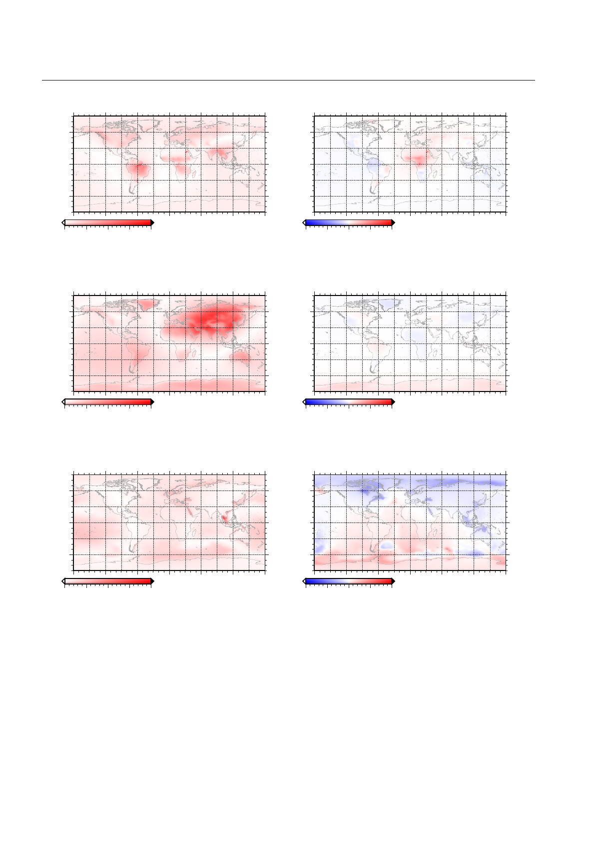
Fig. 1

Annual signals and long-term trends in terrestrial water storage, atmospheric pressure, and ocean loading as given in

the ESMGFZ model; computed between 1979.0 and 2018.0 as 0.5

◦×

0.5

◦

grid; please note the different scales for continental

hydrosphere

4 M¨annel et al.

and Dobslaw (2013). The calculations are performed in

the spatial domain on 0.125

◦×

0.125

◦

global grids in

the near-field (0

◦

- 3.5

◦

) and on 2.0

◦×

2.0

◦

grids in

the far-field (3.5

◦

- 180

◦

) by using mass distributions

provided by the deterministic numerical weather predic-

tion model of the European Centre for Medium-range

Weather Forecasts (ECMWF), the Max-Planck-Institute

for Meteorology Ocean Model (MPIOM, Jungclaus et al,

2013), and the Land Surface Discharge Model (LSDM,

Dill, 2008). The re-mapping applied to all datasets to

arrive at the 0.125

◦

resolution required for the near-field

calculations is described in Dill et al (2018). Based on

global load Love numbers taken from the elastic Earth

model ak135 (Kennett et al, 1995), the surface defor-

mations are provided in two different frames, namely

center of the Earth’s figure (CF) and center of Earth’s

mass (CM). Atmospheric, oceanic, and hydrospheric

loading surface deformations in north, east, and up are

provided with a spatial resolution of 0.5

◦

and a temporal

sampling of three hours for atmosphere and ocean, and

24 h for the continental hydrosphere, (Dill and Dobslaw,

2013). For operational users, the ESMGFZ products are

updated daily at 10:00 UTC, and even provide forecasts

for up to six days into the future based on the routine

numerical weather forecasts issued by ECMWF. In view

of the GGOS consistency goals, it should be mentioned

that ESMGFZ is also providing background models for

satellite gravimetry (AOD1B; Dobslaw et al, 2017) and

Earth orientation excitation functions (EAM; Dobslaw

et al, 2010) that are each based on identical mass dis-

tributions as the surface loading deformations. Figure 1

shows the deformations in vertical direction character-

ized by their annual amplitude (figures a, c, e) and by

their secular trend (figures b, d, f ) for non-tidal continen-

tal hydrosphere (top), atmospheric pressure (middle),

and ocean loading (bottom). Both quantities, the annual

amplitude

and the linear trend

, are determined

by applying a least squares fit:

C(t) =

i=1

Aisin 2π

(t−t0) + φi+b0+b1(t−t0).(1)

In Eqn. 1, the annual period is indicated by

, the

time epoch

is given by January 1st. Parameters

φi

and

specify the phase shifts and the coordinate at

reference epoch J2000.0, respectively. Annual ampli-

tudes (see left part of Figure 1) reach more than 30 mm

for the continental hydrosphere, highlighting the ma-

jor river basins like Amazon, Parana, Congo, Yangtze,

and Ganges. Large scale variation patterns are also visi-

ble in North America, Eurasia, and Africa with annual

amplitudes of up to 5 mm. Atmospheric pressure load-

ing exceeds 10 mm particularly in regions of long-term

stable air pressure regimes like in the interior of Eura-

sia, Antarctica, and Greenland. Non-tidal ocean loading

reaches amplitudes of 10 mm only in some semi-enclosed

seas in Southeast Asia. The right column of Figure 1

shows regional long-term trends in the vertical defor-

mations. In general, positive trends are associated with

decreasing surface loads. Deformations related to at-

mospheric and ocean loading are always smaller than

0.1 mm/a with, in general, large-scale patterns. Trends

in deformations related to continental hydrosphere are

substantially larger and more spatially heterogeneous.

Significantly positive annual uplift rates of up to 1 mm/a

are found for several regions. Most prominent are the

positive trends (i.e. decreased loading) in central Africa,

South America, and the northwest part of Greenland.

Negative trends associated with increased surface load-

ing and associated station subsidence are visible in the

Amazon region, Western US, and West Australia. It is

worth to be mentioned that also very local effects can

create strong trends, as visible for the region of the Lake

Nasser in Egypt (Figure 1(b)).

3 GNSS and VLBI data processing

In order to (1) compare the surface deformations given

in the models against station coordinate time series

as well as to (2) assess potential improvements in e.g.

velocity estimation, both global GNSS (actually GPS-

only) and VLBI datasets were analyzed. GNSS observa-

tions were processed with the GFZ software EPOS.P8

in both network and precise point positioning (PPP)

mode. In general, the GNSS processing followed the

IERS 2010 Conventions (Petit and Luzum, 2010) and

was performed in the ITRF2014 reference frame (Al-

tamimi et al, 2016).

The GNSS network solution was set up similar to the

GFZ IGS rapid processing, i.e. including the estimation

of orbit and Earth rotation parameters. A network of

156 globally distributed stations was selected with data

from the period 2008.0 to 2018.0. For the implications

of using a Global Mapping Function when investigating

loading effects we refer to Steigenberger et al (2009).

The GNSS PPP-solution comprises in total 484 stations

for the time period 2008.8 to 2017.1. Orbit and clock

products are taken from a GFZ internal reprocessing

effort which was set up similar to the configuration of

GFZ official IGS products. However, as the a priori

products used in the PPP processing were computed

without applying surface loading corrections the effect

of surface loading is not fully considered (the impact of

surface loading on satellite orbits is discussed in Sect. 5).

Loading more pages...