remote sensing
Article
Alternative Approach for Tsunami Early Warning Indicated by
Gravity Wave Effects on Ionosphere
Zahra Foroodi 1, Mahdi Alizadeh 1,2,* , Harald Schuh 2,3 and Lung-Chih Tsai 4,5
Citation: Foroodi, Z.; Alizadeh, M.;
Schuh, H.; Tsai, L.-C. Alternative
Approach for Tsunami Early Warning
Indicated by Gravity Wave Effects on
Ionosphere. Remote Sens. 2021,13,
2150. https://doi.org/10.3390/
rs13112150
Academic Editors: Teodosio Lacava,
Mariano Lisi, Katsumi Hattori,
Nicola Genzano and Rossana Paciello
Received: 31 March 2021
Accepted: 24 May 2021
Published: 30 May 2021
Publisher’s Note: MDPI stays neutral
with regard to jurisdictional claims in
published maps and institutional affil-
iations.
Copyright: © 2021 by the authors.
Licensee MDPI, Basel, Switzerland.
This article is an open access article
distributed under the terms and
conditions of the Creative Commons
Attribution (CC BY) license (https://
creativecommons.org/licenses/by/
4.0/).
1Faculty of Geodesy and Geomatics Engineering, K. N. Toosi University of Technology, 19697 Tehran, Iran;
2German Research Centre for Geosciences (GFZ), 14473 Potsdam, Germany; [email protected]
3Institute of Geodesy and Geoinformation Sciences, Technical University of Berlin, 10553 Berlin, Germany
4GPS Application and Research Center, National Central University, Taoyuan 320317, Taiwan;
lctsai@csrsr.ncu.edu.tw
5Center for Space and Remote Sensing Research, National Central University, Taoyuan 320317, Taiwan
*Correspondence: [email protected]
Abstract:
The rapid displacement of the ocean floor during large ocean earthquakes or volcanic
eruptions causes the propagation of tsunami waves on the surface of the ocean, and consequently
internal gravity waves (IGWs) in the atmosphere. IGWs pierce through the troposphere and into
the ionospheric layer. In addition to transferring energy to the ionosphere, they cause significant
variations in ionospheric parameters, so they have considerable effects on the propagation of radio
waves through this dispersive medium. In this study, double-frequency measurements of the Global
Positioning System (GPS) and ionosonde data were used to determine the ionospheric disturbances
and irregularities in response to the tsunami induced by the 2011 Tohoku earthquake. The critical
frequency of the F2 layer (foF
2
) data obtained from the ionosonde data also showed clear disturbances
that were consistent with the GPS observations. IGWs and tsunami waves have similar propagation
properties, and IGWs were detected about 25 min faster than tsunami waves in GPS ground stations
at the United States west coast, located about 7900 km away from the tsunami’s epicenter. As IGWs
have a high vertical propagation velocity, and propagate obliquely into the atmosphere, IGWs can
also be used for tsunami early warning. To further investigate the spatial variation in ionospheric
electron density (IED), ionospheric profiles from FORMOSAT-3/COSMIC (F3/C) satellites were
investigated for both reference and observation periods. During the tsunami, the reduction in IED
started from 200 km and continued up to 272 km altitude. The minimum observed reduction was
2.68
×
10
5
el/cm
3
, which has happened at 222 km altitude. The IED increased up to 767 km altitude
continuously, such that the maximum increase was 3.77 ×10⁵el/cm3at 355 km altitude.
Keywords: ionospheric disturbances; tsunami; internal gravity waves; vertical coupling
1. Introduction
Based on the electric charge, the Earth’s atmosphere is divided into two major layers,
the troposphere and the ionosphere. The troposphere, in which the atmospheric compo-
nents are electrically neutral, is the lower atmosphere ranging from the surface to about
60 km [
1
]. The ionosphere is the upper part of the Earth’s atmosphere, which is extended
from approximately 60 km to more than 1000 km. Solar radiation produces free electrons
and ions in this region that affect the propagation of electromagnetic waves [
2
]. Studying
the coupling between these two layers has been an interesting topic for atmosphere and
space weather research for several decades [
3
]. A tsunami displaces the atmosphere as
it propagates across the open ocean, the atmosphere responds to this excitation by prop-
agating gravity waves obliquely upward, these waves are referred to as internal gravity
waves (IGWs), and grow nearly exponentially with height as they proceed into the rarefied
regions of the upper atmosphere [
4
]. IGWs are buoyancy oscillations that can propagate
Remote Sens. 2021,13, 2150. https://doi.org/10.3390/rs13112150 https://www.mdpi.com/journal/remotesensing

Remote Sens. 2021,13, 2150 2 of 21
horizontally and vertically, their propagation is under the gravity force of the Earth [
5
].
On the one hand, the ionospheric disturbances can decrease the performance of precise
positioning and navigation [
6
]. On the other hand, the ionospheric disturbance signals
induced by some tropospheric events, such as earthquakes, tsunamis, and lightning, can
be used to study these events [7–9].
A tsunami is generated when a large oceanic earthquake or volcanic eruption causes
rapid displacement of the ocean floor. Studies about the propagation of IGWs during the
1970s have suggested that the ionosphere is sensitive to IGWs by the forcing effect of a
tsunami on the surrounding atmosphere [
10
]. Peltier and Hines inferred that IGWs might
be detectable and used for tsunami warning system purposes [
4
]. After the Sumatra and
Indian tsunami in 2004, researchers pay significant attention to observing tsunamis by
ionospheric sounding. Using the high-frequency Doppler sounding network in Taiwan, Liu
et al. observed ionospheric disturbances triggered by the 2004 Indian Ocean tsunami [
11
].
Occhipinti et al. used total electron content (TEC) data measured by the Jason-1 and
Topex/Poseidon satellite altimeters to detect the signature of IGWs on the ionosphere [
12
].
However, both Doppler sounding networks and altimetry satellites have a low spatial and
temporal resolution, which makes it difficult to study the propagation characteristics of
ionospheric disturbances in detail. Artru et al. used TEC data, observed from the Geonet
network in Japan, to extract the ionospheric disturbances induced by the 23 June 2001
8.2 Mw earthquake in Peru for the first time [
8
]. Due to the high spatial and temporal
resolution, the GPS TEC data have been widely used in ionospheric monitoring and
tsunami detection [13–16].
According to the US Geological Survey, an earthquake (Mw = 9) occurred with the
epicenter at 38.32
◦
N, 142.37
◦
E; it occurred on 11 March 2011 at 5:46:23 UT near Tohoku,
Japan, and then induced a tsunami. In this paper, we employ various geodetic techniques
to detect ionospheric disturbances and ionospheric irregularities induced by the tsunami
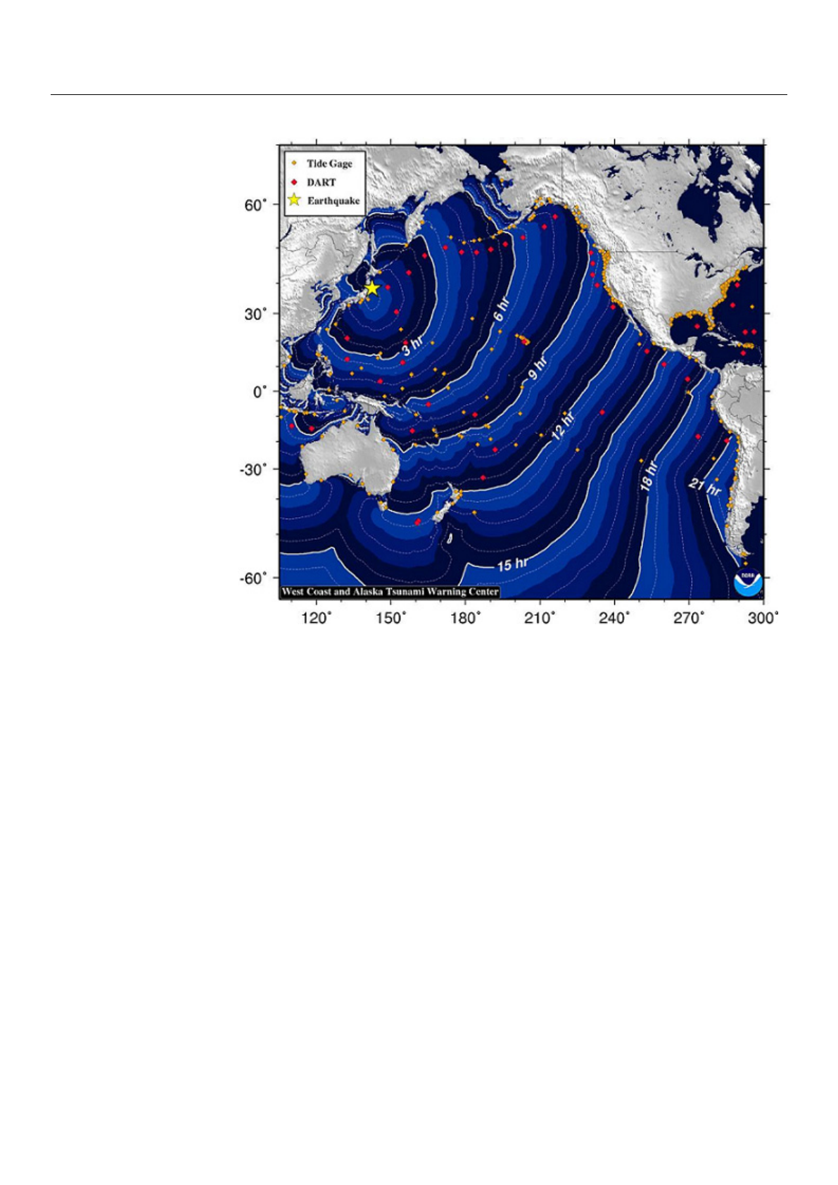
on the west coast of the United States of America. According to the travel time map in
Figure 1, the tsunami reached the west coast of the USA about 10 h after the earthquake.
Various researchers have studied the arrival time of IGWs in the 2011 Tohoku tsunami, but
their approach was mainly post-process. In this paper we investigated a near real-time
method to detect IGWs, therefore using this procedure can lead to faster tsunami warnings
compared to DARTs and tide gauges. Moreover, ionospheric perturbations caused by
tsunamis were also studied by different satellite geodetic techniques.
Remote Sens. 2021,13, 2150 3 of 21
Remote Sens. 2021, 13, x FOR PEER REVIEW 3 of 23
Figure 1. Travel time map of the 2011 Tohoku tsunami. The spatial distribution of tide gauge (or-
ange point), DART (red point), and location of the epicenter (yellow star) are shown in the figure
[17].
2. Materials
In this study, 56 GPS stations were selected from the UNAVCO network,
(http://www.unavco.org/data/gps-gnss.html- accessed on 20 April 2020 ). The sampling
interval for all stations was 15 s or 30 s. To identify the peculiar signatures of the iono-
sphere during the tsunami, data of one day before and one day after the tsunami day were
analyzed. Data from ionosonde, the deep-ocean assessment and reporting of tsunamis
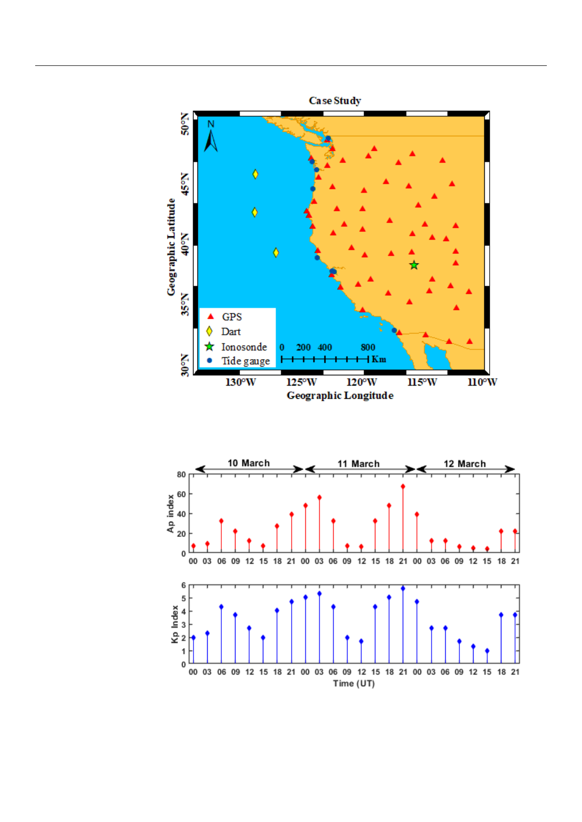
(DART), and tide gauges were used to validate the obtained results. Figure 2 shows the
spatial distribution of the stations and the types of instruments used in the present analy-
sis.
Figure 1.
Travel time map of the 2011 Tohoku tsunami. The spatial distribution of tide gauge (orange
point), DART (red point), and location of the epicenter (yellow star) are shown in the figure [17].
2. Materials
In this study, 56 GPS stations were selected from the UNAVCO network, (http://
www.unavco.org/data/gps-gnss.html, accessed on 20 April 2020). The sampling interval
for all stations was 15 s or 30 s. To identify the peculiar signatures of the ionosphere during
the tsunami, data of one day before and one day after the tsunami day were analyzed. Data
from ionosonde, the deep-ocean assessment and reporting of tsunamis (DART), and tide
gauges were used to validate the obtained results. Figure 2shows the spatial distribution
of the stations and the types of instruments used in the present analysis.
Solar and geomagnetic activities are the dominating factors that control the behavior
of the ionosphere. Geomagnetic storms and solar activity mask the effects of tropospheric
events in the ionosphere, and responses of the F region to tsunamis can be sought only
under particular geomagnetic and solar conditions [
18
]. The index F10.7 was 129.5, 121.5,
and 119.2 solar flux units (SFU) on 10, 11, and 12 March, respectively. According to the F10.7
index variation, solar radiation was in the steady state. The geomagnetic activity can be
interpreted using several parameters. One of these parameters is the Kp index, which varies
from 0 to 9 (values equal and greater than 5 represent a geomagnetic storm) [
19
]. Another
parameter is the Ap index, which varies from 0 to 400 (values greater than 50 represent
a geomagnetic storm) [
20
]. Figure 3shows the geomagnetic activity level. The solar and
geomagnetic indices were downloaded from the archives of Goddard Space Flight Center
(https://omniweb.gsfc.nasa.gov/form/dx1.html, accessed on 20 April 2020).
Remote Sens. 2021,13, 2150 4 of 21
Remote Sens. 2021, 13, x FOR PEER REVIEW 4 of 23
Figure 2. Case study and the spatial distribution of ground-based GPS receivers (red triangle),
DART stations (yellow diamond), tide gauge stations (dark-blue circle), and ionosonde station
(green asterisk) considered in this study.
Solar and geomagnetic activities are the dominating factors that control the behavior
of the ionosphere. Geomagnetic storms and solar activity mask the effects of tropospheric
events in the ionosphere, and responses of the F region to tsunamis can be sought only
under particular geomagnetic and solar conditions [18]. The index F10.7 was 129.5, 121.5,
and 119.2 solar flux units (SFU) on 10, 11, and 12 March, respectively. According to the
F10.7 index variation, solar radiation was in the steady state. The geomagnetic activity can
be interpreted using several parameters. One of these parameters is the Kp index, which
varies from 0 to 9 (values equal and greater than 5 represent a geomagnetic storm) [19].
Another parameter is the Ap index, which varies from 0 to 400 (values greater than 50
represent a geomagnetic storm) [20]. Figure 3 shows the geomagnetic activity level. The
solar and geomagnetic indices were downloaded from the archives of Goddard Space
Flight Center (https://omniweb.gsfc.nasa.gov/form/dx1.html- accessed on 20 April 2020).
Figure 2.
Case study and the spatial distribution of ground-based GPS receivers (red triangle),
DART stations (yellow diamond), tide gauge stations (dark-blue circle), and ionosonde station (green
asterisk) considered in this study.
Remote Sens. 2021, 13, x FOR PEER REVIEW 5 of 23
Figure 3. Geomagnetic conditions during 10–12 March 2011.
Referring to Figure 3, the Kp index was below 5 units on March 11, from 6 to 18 UT,
which indicates quiet geomagnetic conditions during the major part of the tsunami event.
3. Methods
3.1. TEC Measurements
Using dual-frequency GPS observations ( 1
f
= 1575.42 MHz, 2
f
= 1227.60 MHz), the
ionospheric delay can be calculated. Then smoothed code pseudorange measurements for
1
f
and 2
f
are estimated using the following Equation (1) [21]:
2
2
1, 1,i 1, 1, 1, 2, 1, 2,
22
12
2
1
2,2,i2,2, 1,2, 1,2,
22
12
2( ( ))
2( ( ))
k kkk kk kk
iii iiii
kkkk kk kk
iii iiii
f
PPLL LL LL
ff
f
PPLL LL LL
ff
=+−+ −− −
−
=+−+ −− −
−
(1)
where k and i denote the pseudo-random noise (PRN) of a given satellite and receiver,
respectively; 1,
k
i
P
and 2,
k
i
P
are the smoothed dual-frequency code measurements at epoch
t; 1,
k
i
Land 2,
k
i
Lare the phase measurements observed by receiver i as seen from satellite
k at epoch t; 1,
k
i
L and 2,
k
i
Lare the mean phase measurements at cycle slip free time in-
terval; 1,i
k
P and 2,i
k
P are the mean code measurements. Finally, slant TEC (STEC) value
is calculated using the following equation:
22
12
,4
22
21
() ( () )
40.31( )
kkk
iiiL
ff
STEC t P t DCB DCB
ff
ε
=−−+
−
. (2)
In Equation (2) ()
k
i
STEC t is slant TEC between satellite k and receiver i, ,4 ()
k
i
Pt
is the smoothed code measurement, or the so-called geometry-free linear combination.
k
DCB and i
DCB denote the satellite and receiver differential code biases, respec-
tively. In this study, i
DCB value is calculated using the Li et al. method [22]. In this
Figure 3. Geomagnetic conditions during 10–12 March 2011.
Referring to Figure 3, the Kp index was below 5 units on March 11, from 6 to 18 UT,
which indicates quiet geomagnetic conditions during the major part of the tsunami event.

Remote Sens. 2021,13, 2150 5 of 21
3. Methods
3.1. TEC Measurements
Using dual-frequency GPS observations (
f1
= 1575.42 MHz,
f2
= 1227.60 MHz), the
ionospheric delay can be calculated. Then smoothed code pseudorange measurements for
f1and f2are estimated using the following Equation (1) [21]:
e
Pk
1,i=Pk
1,i+Lk
1,i−Lk
1,i+2f2
2
f2
1−f2
2
(Lk
1,i−Lk
2,i−(Lk
1,i−Lk
2,i))
e
Pk
2,i=Pk
2,i+Lk
2,i−Lk
2,i+2f2
1
f2
1−f2
2
(Lk
1,i−Lk
2,i−(Lk
1,i−Lk
2,i)) (1)
where kand idenote the pseudo-random noise (PRN) of a given satellite and receiver,
respectively;
e
Pk
1,i
and
e
Pk
2,i
are the smoothed dual-frequency code measurements at epoch t;
Lk
1,i
and
Lk
2,i
are the phase measurements observed by receiver ias seen from satellite kat
epoch t;
Lk
1,i
and
Lk
2,i
are the mean phase measurements at cycle slip free time interval;
Pk
1,i
and
Pk
2,i
are the mean code measurements. Finally, slant TEC (STEC) value is calculated
using the following equation:
STECk
i(t) = f2
1f2
2
40.31(f2
2−f2
1)(e
Pk
i,4(t)−DCBk−DCBi+εL)(2)
In Equation (2)
STECk
i(t)
is slant TEC between satellite kand receiver i,
e
Pk
i,4(t)
is the
smoothed code measurement, or the so-called geometry-free linear combination.
DCBk
and
DCBi
denote the satellite and receiver differential code biases, respectively. In this
study,
DCBi
value is calculated using the Li et al. method [
22
]. In this method, the global
ionospheric map (GIM) TEC values are interpolated to the same GPS footprint locations
and times. The
DCBi
of each station is estimated by least squares adjustment using the
observations of all satellites. To remove multipath effects, only the measurements with
elevation angles higher than 20
◦
are considered. STEC along the GPS line of sight (LOS) is
converted into the vertical TEC (VTEC) using the mapping function as follows:
VTEC =STEC cos(sin−1(Resin z
Re+Hion
)) (3)
where
Re
represents the mean radius of the Earth,
z
is the zenith distance of the LOS from
the receiver to GPS satellites, and
Hion
is the altitude of the ionospheric thin-layer shell,
which is set to 450 km in this study.
3.2. TEC Disturbances
Hernández-Pajares et al., Ref. [
23
], used a first-order numerical difference method to
extract ionospheric disturbances. Their method uses Equation (4), as follows:
∆TEC(t) = ∆s(t) = s(t)−0.5(s(t−τ) + s(t+τ)) (4)
where
∆s(t)
is the first-order numerical difference of TEC series, tand
τ
denote the ob-
servation epoch and time step, respectively. This method can effectively capture the TEC
variations for measurements with elevation angle higher than 40
◦
. In this paper, a second-
order numerical difference method is employed to eliminate the TEC trend because the
satellites at low elevation can better highlight the presence of oscillating perturbations [
12
].
The second-order numerical difference is calculated by Equation (5), as follows:
∆2TEC(t) = ∆2S(t) = ∆S(t)−1
2(∆S(t−τ) + ∆S(t+τ)) (5)
The
∆2S(t)
values and primary IGW signals have the same period (
T
), and the ratio
amplitude (R) is calculated using Equation (6), as follows:
Loading more pages...