Emergent collective dynamics of pusher and puller squirmer rods: swarming, clustering, and turbulence [original]

This journal is © The Royal Society of Chemistry 2022 Soft Matter, 2022, 18, 6179–6191 | 6179

Cite this: Soft Matter, 2022,

18, 6179

Emergent collective dynamics of pusher and

puller squirmer rods: swarming, clustering,

and turbulence†

Arne W. Zantop * and Holger Stark *

We study the interplay of steric and hydrodynamic interactions in suspensions of elongated micro-

swimmers by simulating the full hydrodynamics of squirmer rods in the quasi two-dimensional geometry

of a Hele-Shaw cell. To create pusher or puller-type squirmer rods, we concentrate the surface

slip-velocity field more to the back or to the front of the rod and thereby are able to tune the rod’s

force-dipole strength. We study a wide range of aspect ratios and area fractions and provide

corresponding state diagrams. The flow field of pusher-type squirmer rods destabilizes ordered

structures and favors the disordered state at small area fractions and aspect ratios. Only when steric

interactions become relevant, we observe a turbulent and dynamic cluster state, while for large aspect

ratios a single swarm and jammed cluster occurs. The power spectrum of the turbulent state shows two

distinct energy cascades at small and large wave numbers with power-law scaling and non-universal

exponents. Pullers show a strong tendency to form swarms instead of the disordered state found for

neutral and pusher rods. At large area fractions a dynamic cluster is observed and at larger aspect ratio a

single swarm or jammed cluster occurs.

1 Introduction

Microscopic unicellular organisms make up a major fraction of

all life forms on our planet. They are involved in important

natural processes such as photosynthesis

1–3

or industrial pro-

cesses such as the production of enzymes

4,5

or biofuels,

6–8

the recycling of wastewater.

9,10

Especially in photosynthesis,

commonly viewed as the basis of life, unicellular phytoplankton

accomplish about half of the worldwide natural turnover.

2,3

However, still many aspects of the behavior of unicellular

organisms is not completely understood. In fact, many of these

life forms are self-propelling microswimmers,

11–13

as, for exam-

ple, the algae C. reinhardtii

14,15

or the bacterium E. coli.

16–18

From the perspective of physicists, their active motion gives rise

to very interesting new collective phenomena. In this article we

study the rich emergent collective dynamics of rod-shaped

model microswimmers, which we can tune between the pusher

and puller type.

Active motion is always performed in non-equilibrium and,

therefore, gives rise to new and interesting phenomena. For

example, specially designed boundaries can rectify the random

motion of active particles,

19–23

or under gravity active particles

develop polar order and even show inverted sedimentation

profiles when they are bottom-heavy.

24,25

In addition, micro-

swimmer suspensions are subject to long-range hydrodynamic

interactions with characteristic power-law decay.

13,26,27

But also

short-range steric interactions play an important role, in parti-

cular, for elongated particles, which align along each other.

The combination of these interactions gives rise to numerous

interesting dynamic patterns. Common examples are the for-

mation of swarms or flocks,

28–32

convection rolls and plumes,

fluid pumps,

33,34

vortices,

35–38

active nematic patterns,

39–41

and

the emergence of the so-called active turbulence,

42,43

termed in

analogy to classical inertial turbulence.

44,45

However, contrary to

classical turbulence, where fluid flow is driven on the macroscopic

scale, active turbulence is generated at the microscopic scale of

the self-propelled particles and then energy is dissipated on larger

scales. This mechanism causes a characteristic length scale for

the formation of vortices and patterns, which is in contrast to

the scale invariance of classical turbulence.

46–48

In particular, the

specific model parameters now determine the scaling of the

velocity power spectrum, which is no longer universal.

48–50

Active

turbulence is found for microswimmers,

51,52

active bio-filaments,

which exist in the cytoplasm,

39,53

and in growing tissue.

54,55

Institut fu

¨r Theoretische Physik, Technische Universita

¨t Berlin, Hardenbergstraße 36,

10623 Berlin, Germany. E-mail: a.zantop@tu-berlin.de, holger.s[email protected]

†Electronic supplementary information (ESI) available: We provide eight videos

of diﬀerent collective dynamic states in the top view. Videos 1–3 show pusher rods

in the turbulent (1), single swarm (2) and dynamic cluster state (3). Videos 4–8

show puller rods in the swarming (4 and 8), single swarm (5), jammed cluster (6),

and dynamic cluster state (7). See DOI: https://doi.org/10.1039/d2sm00449f

Received 8th April 2022,

Accepted 30th June 2022

DOI: 10.1039/d2sm00449f

rsc.li/soft-matter-journal

Soft Matter

PAPER

Open Access Article. Published on 05 July 2022. Downloaded on 10/27/2022 10:58:01 AM.

This article is licensed under a

Creative Commons Attribution 3.0 Unported Licence.

View Article Online

View Journal

| View Issue

6180 | Soft Matter, 2022, 18, 6179–6191 This journal is © The Royal Society of Chemistry 2022

On the theoretical side, the dynamics of active particles has

been investigated at diﬀerent levels of description. While the

celebrated Vicsek model

56–58

uses coarse-grained alignment

rules, also models with explicit steric interactions exist.

42,51,59–64

Thesemodelshavealsobeengeneralizedtoactivefilaments

31,65,66

and models, which implicitly include hydrodynamic inter-

actions.

67,68

Models, which directly simulate fluid flow and

thereby explicitly include hydrodynamic interactions, use the

method of multi-particle collision dynamics (MPCD)

25,30,32,69–79

or the lattice-Boltzmann method.

80–83

Continuum models

combine elements of the Toner-Tu

and Swift-Hohenberg

equations to generate hydrodynamic equations for active

suspensions.

46,86,87

Microswimmers are also distinguished by

their swimming mechanisms and the flow field, they generate

in the surrounding fluid.

11,13

While some microorganisms

propel with cilia located all over their surface, common bacteria

and algae propel with flagella that extent from the front or back

of the cell body. In the first case, the flow field of a source

dipole is realized, which decays as r

3

, while bacteria and algae

are termed pusher or puller-type swimmers that generate a

long-range force-dipole flow field, which decays as r

2

13,27

The

specific form of these hydrodynamic multipole flow fields deter-

mines the collective dynamics of the microswimmers.

32,69,74,88–90

In this context, we proposed in ref. 76 the squirmer rod as

a realistic microscopic model for elongated microswimmers.

It consists of overlapping squirmers and thereby extends the

well-known spherical squirmer model for ciliary propulsion

26,91

and its implementation in MPCD.

Restricting the surface slip-

velocity to the front or the back of the squirmer rod, puller and

pusher-type squirmer rods can be realized, respectively. The

hydrodynamic flow field is simulated using an eﬃcient imple-

mentation of MPCD with a reduced compressibility such that

also collective dynamics in large and dense systems can be

studied.

Most recently, we presented the state diagram of

neutral squirmer rods and identified with increasing area

fraction and depending on the aspect ratio of the rods the

disordered state, dynamic swarms, a single swarm, and ultimately

ajammedcluster.

In this article we generalize the squirmer-rod model to

pushers and pullers with tunable force-dipole strength in the

flow field. Compared to spheroidal squirmers it has the advan-

tage that it better approximates real rodlike microswimmers

such as E. coli. Using this model, we provide a comprehensive

study of the state diagram for hydrodynamically interacting

microswimmers over a wide range of aspect ratios, densities,

and force-dipole strengths as the state diagrams in Fig. 3(a),

7(a) and 9(a) show. Hereby, we go well beyond previous works,

which focused mainly on more dilute systems

95,96

or a single

aspect ratio.

Thus, our work provides an overall view how

hydrodynamics and shape determine the dynamic states of

microswimmers. For example, our particle-based model nicely

illustrates that the active turbulent state occurs as a compro-

mise between the disordering hydrodynamic pusher–pusher

interactions and aligning steric interactions. We also demon-

strate that the two distinct energy cascades at low and large

wave numbers in the power spectral density of velocity

fluctuations exhibits non-universal exponents. Moreover, we

find a dynamic cluster state at large densities. Besides this

state all other states are also found in dry active rods.

But, in

our case, they have a specific contribution from hydrodynamics

as, for example, the turbulent and swarming states show. The

overall appearance of the states in our state diagrams can be

summarized as follows. For pushers we observe that the swarm-

ing states of neutral squirmer rods are destabilized. Instead, for

smaller aspect ratio between the disordered and dynamic

cluster state, we observe the turbulent state as already men-

tioned. At high aspect ratios, where steric interactions become

more relevant, we recover the single swarm and jammed cluster

state of neutral squirmer rods. For pullers, hydrodynamic

interactions stabilize the swarming state even for our smallest

area fraction. Thus, compared to neutral squirmer rods, states

are shifted towards lower densities. Variation of the force-dipole

strength at constant aspect ratio supports all these findings.

The article is organized as follows. In Section 2 we give a

brief overview of the methods used in this paper. Section 3

provides a detailed study of the diﬀerent dynamic states of the

squirmer rods as a function of their area fraction, aspect ratio,

and force-dipole strength. We end with a summary and con-

clusions in Section 4.

2 System and methods

We first introduce the squirmer-rod model and then summarize

some details of the method of multi-particle collision dynamics,

which we use to simulate the flow fields generated by the

squirmer rods.

2.1 Model of the squirmer rod

To model shape-anisotropic microswimmers, we employ the

squirmer rod model as introduced in our previous work.

Squirmer rods consist of N

overlapping spherical squirmers

of radius R

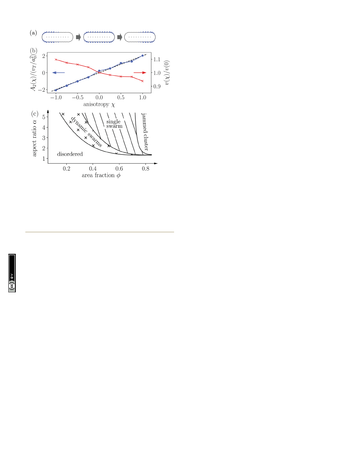
, arranged on a line to form a single rigid body [see

Fig. 1(a)]. By varying the distance dbetween neighboring

squirmers, we can tune the aspect ratio of the squirmer rod,

a=l

/2R, where l

is the rod length. However, we do not exceed

a distance of dE0.8Rso that the surface of the rod is

suﬃciently smooth. With a number of N

= 10 squirmers in

this work, this amounts to a maximum aspect ratio of aE5,

which closely resembles the aspect ratio of bacteria such as

E. coli or B. subtilis.

The squirmer rods propel through the axisymmetric and

tangential slip velocity field at the surface of individual sphe-

rical squirmers,

[(e

ˆxˆ

)xˆ

e

ˆ], (1)

which is imposed on the surrounding fluid.

26,92

Here, e

ˆis the

rod axis and xˆ

the unit vector pointing from the center of a

squirmer to a point on the squirmer surface. This generates a

source-dipole flow field, which is a higher-order singular

solution of the Stokes equations Zr

v=rptogether with the

incompressibility condition rv= 0, that govern fluid flow at

Paper Soft Matter

Open Access Article. Published on 05 July 2022. Downloaded on 10/27/2022 10:58:01 AM.

This article is licensed under a

Creative Commons Attribution 3.0 Unported Licence.

View Article Online

This journal is © The Royal Society of Chemistry 2022 Soft Matter, 2022, 18, 6179–6191 | 6181

the microscale. Here, vand pare the respective fluid velocity

and pressure fields, and Zis the dynamic shear viscosity. The

strength B

controls the swimming velocity v

= 2/3B

of the

spherical squirmer and hence of the squirmer rod. In ref. 76

we showed that the swimming velocity of the squirmer rods

vE1.2v

slightly exceeds the velocity of a single spherical

squirmer. Additionally, the velocity of the rods varies by 10% in

the range of aspect ratios used in this article. Although the

increased velocity at the larger aspect ratios might augment

clustering, we assume the eﬀect to be negligible.

As described so far, the surface slip velocity of the squirmer

rod resembles ciliated microorganisms such as Paramecium.

In this realization, the profile of the slip velocity generates a

flow field in the surrounding fluid, the far field of which can be

described by a source dipole and an additional force quadru-

pole singularity, which both decay with |u

|, |u

|Br

3

,aswe

show in ref. 76.

However, other prominent microswimmers such as E. coli

bacteria or Chlamydomonas algae propel by rotating or beating

flagella that extent from the back or the front of their bodies,

respectively. These modes of propulsion create a pair of oppos-

ing forces that generate the more long-ranged force-dipole flow

field |u

|Br

2

. To generalise the squirmer rod model to these

pusher and puller-type microswimmers, we concentrate the

surface slip velocity either to the back or the front of the

squirmer rod [see Fig. 1(a)]. This is done by multiplying

the surface flow field with the envelope function

fðx

s^

e;wÞ¼1þwtanhð10x

s^

e=lSÞ;(2)

where x

spoints from the rod center to a location on the rod

surface. The parameter wA[1, 1] determines the swimmer

type and force-dipole strength, such that for wo0 a pusher-

type swimmer is realised and likewise a puller-type swimmer

for w40. For either w=1orw= 1 this modification leads to a

completely passive half of the rods [see Fig. 1(a)], while for

intermediate values the relative contributions of the source

dipole and force dipole to the flow field vary. For w= 0, the

model again resembles the neutral squirmer rod.

In the present work, we consider the collective dynamics of

squirmer rods confined between two parallel walls. In this

so-called Hele-Shaw cell the radial decays of hydrodynamic

multipoles are modified compared to the bulk fluid, such that

theconfinedsourcedipoleandforcedipoledecayas|u

|Br

2

and |u

|Br

3

, respectively, where ris the polar distance

76,99

(see

appendix of ref. 99). As a consequence, the source dipole has the

longest range in the flow field and ultimately dominates the far

field. However, already in our previous work we realized that a

distance of Dz=6Rbetween the walls, which we will use in our

simulations, alters the relative strength of the source and force

dipoles.

As a consequence, the force dipole dominates the flow

field at short and medium distance as we will demonstrate in

Section 3.2.

2.2 Method of multi-particle collision dynamics

To model the fluid flow in our simulations, we employ the

meso-scale simulation technique of multi-particle collision

dynamics (MPCD).

100–102

The MPCD method is particularly

suited for solving the Navier–Stokes equations at the micro-

scale, because it includes thermal fluctuations and is straight-

forward to implement boundary conditions for complex

geometries.

The MPCD method uses a sequence of streaming and

collision steps of the point-like fluid particles. In the streaming

step the fluid particles move ballistically with their velocities

during time step Dt. Then, the simulation box is divided into

cubic cells with edge length a

and the velocities of the fluid

particles in one cell are modified randomly but keeping the

mean velocity or linear momentum fixed. In this work, we use a

collision rule optimized to achieve a low compressibility of the

fluid.

As in other MPCD methods, it includes angular

momentum conservation and a thermostat. By choosing the

MPCD fluid density n

= 20/a

,i.e., on average 20 fluid particles

per cell, and the time step Dt¼0:005a0ﬃﬃﬃﬃﬃﬃﬃﬃﬃﬃﬃﬃﬃﬃﬃﬃﬃﬃﬃ

m0=kBT0

p, we obtain a

fluid viscosity of Z¼16:05 ﬃﬃﬃﬃﬃﬃﬃﬃﬃﬃﬃﬃﬃﬃﬃﬃ

m0kBT0

p=a0

2, which is comparable

to previous work.

74,76,96

Here, m

is the mass of one fluid

particle.

The immersed squirmer rods are modeled with the mass

density of the fluid r

. The radius of the constituting

squirmersischosenasR

=3a

and the strength of the surface slip

velocity as B

=0.1,whichresultsinaPe

´clet number of Pe E350.

Steric repulsion is realized with a Weeks–Chandler–Andersen

Fig. 1 (a) Sketch of the surface slip velocity of three squirmer rods with

respective swimmer-type parameters w=1, 0, and 1 (from left to right).

The arrows within the squirmer rods indicate the swimming direction e

ˆ.

The parameter wA{1, 1} can be used to smoothly vary the type of the

squirmer rod from pusher to neutral to puller. (b) Force-dipole coeﬃcient

(w) (blue) and active velocity v(w)/v(0) (red) as a function of the swimmer

parameter w. (c) Schematic state diagram for neutral squirmer rods adapted

from ref. 94.

Soft Matter Paper

Open Access Article. Published on 05 July 2022. Downloaded on 10/27/2022 10:58:01 AM.

This article is licensed under a

Creative Commons Attribution 3.0 Unported Licence.

View Article Online

6182 | Soft Matter, 2022, 18, 6179–6191 This journal is © The Royal Society of Chemistry 2022

potential

103

that acts between two squirmers of different rods.

To ensure that there is no significant overlap between two

squirmer rods, we choose a strong force constant e

WCA

E10

The squirmer rods move because they acquire momentum

from the surrounding fluid. In the MPCD streaming step, linear

and angular momentum is transferred to the squirmer rod by

collisions with the fluid particles. We achieve this by applying

the so-called bounce back rule, which we also modify accord-

ingly to implement the slip velocity in eqn (1) on the surface of

the squirmer rods.

100,101

Squirmer rods also contain so-called

‘‘ghost’’ particles, which improve the implementation of no-slip

boundary conditions.

101

During the MPCD collision step, they

exchange momentum with the fluid, which is ascribed to the

squirmer rod. Lastly, the equations of motion for the squirmer

rods are integrated with a refined time step of dt

=Dt/3

using a symplectic splitting algorithm for rigid body molecular

dynamics.

104

For our simulations we use two diﬀerent geometries.

To determine how the force dipole strength A

depends on

the swimmer-type parameter w, we use a cubic box of linear size

L= 100a

with periodic boundary conditions along all spatial

directions. In this case we use the time 10

Dtto equilibrate the

MPCD fluid flow fields and then average the fluctuating flow

fields over additional 5 10

Dttime steps during simulations.

To simulate the collective dynamics of the squirmer rods, we

consider the quasi two-dimensional geometry of a Hele-Shaw

cell of linear size L= 300a

in the xand ydirection. Along the

zdirection the system is confined by walls separated by a

distance Dz=6Rto mimic the experimental setups using

microfluidic chambers

51,105

or liquid–oil interfaces.

106,107

It has

also been used in previous work.

94,97

Additionally, this realization

guarantees a strong contribution of the force-dipole interaction

in the near field, as we will show in Section 3.2 and Fig. 2. In the

xand ydirection periodic boundary conditions are employed.

In this geometry, the Nsquirmer rods are confined to only

move in the midplane of the Hele-Shaw cell by a strong

harmonic potential. The rods’ initial positions are generated

randomly for area fractions f=NA

o0.6, where A

is the

two-dimensional cross section of one squirmer rod. For fZ0.6

squirmer rods are placed on a rectangular lattice, all with a

randomly chosen orientation either parallel or anti-parallel to

one of the major axis of the unit cell. We simulate for a time of

Dtwhile saving snapshots every 2500Dtfor further analysis.

To ensure that the system is equilibrated, we omit the first

100 snapshots from the analysis.

To improve statistics in the study of the emergent turbulent

patterns of pusher-type squirmer rods, we perform two addi-

tional simulation runs for all turbulent states and their neigh-

boring points in the (a,f) parameter space. Furthermore, for all

these cases we also perform three simulation runs with an

increased system size of L= 600a

to investigate finite-size eﬀects.

3 Results

In the following we report on our simulation results. First, we

show that the anisotropy parameter wof the surface slip-velocity

field is directly proportional to the strength of the hydro-

dynamic force-dipole field and we illustrate the flow field of a

single pusher-type squirmer rod in the Hele-Shaw cell. Then, we

thoroughly discuss the state diagrams of the strongest pusher

rod (w=1) and the strongest puller rod (w= 1) depending on

aspect ratio aand area fraction f. We describe the diﬀerent

states using the velocity pair-correlation function, the power

spectral density of the velocity fluctuations, and the orienta-

tional autocorrelation function. Finally, for a specific aspect

ratio a, we show the state diagram in the space of wversus f.

3.1 Variation of the swimmer-type parameter v

To extract the force-dipole coeﬃcient A

from the flow field of

the squirmer rod in the 3D bulk fluid, we follow the method

described in detail in our previous article ref. 76. To do so, we

consider the expansion of an axisymmetric flow field into a

series of hydrodynamic multipoles u(r)=u

(r)+u

(r)+

(r)+..., where the leading-order multipoles are the force

dipole, source dipole, and force quadrupole, respectively. The

radial velocity component with the general form urðr;yÞ¼

n¼1

AnrnþBnrn2



Pnðcos yÞis measured from the simula-

tions and then projected on the second Legendre polynomial

(cosy). From the resulting polynomial 5

2Ðp

0urðr;yÞP2ðcos yÞ

sin ydy¼A2r2þB2r4, we determine the force-dipole

coeﬃcient A

by a polynomial fit in r

1

Indeed, we find a linear relation of the swimmer-type para-

meter wand the force-dipole coeﬃcient wBA

[Fig. 1(b)]. This

is expected since the terminal values of the envelope function

f(x) in eqn (2), which determine the strength of the force

dipole, are linear in w. Furthermore, we find that due to the

definition of the envelope function with hf(x)i= 1, the swim-

ming velocity is nearly independent of w[cf. Fig. 1(b), red curve].

3.2 Force-dipole flow fields in the Hele-Shaw geometry

As already explained, our study of the collective dynamics of the

squirmer rods is performed in a Hele-Shaw cell, which alters

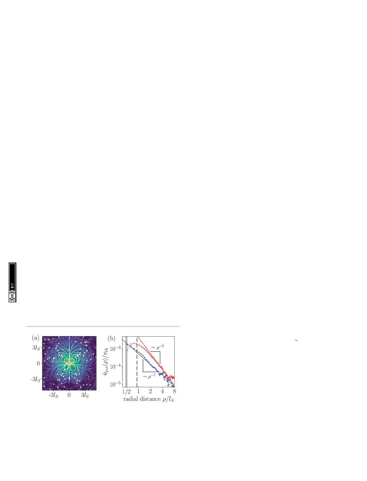
Fig. 2 Hydrodynamic flow field around a pusher-type squirmer rod

(w=1.0) swimming in the Hele-Shaw geometry with cell height Dz=6R.

(a) Flow field in the mid plane of the Hele-Shaw cell. The force dipole clearly

dominates the near field. (b) Radial components u

r,n

(r)oftheleadingsource-

dipole (blue) and force-dipole (red) flow fields. They are normalized by the

thermal velocity of fluid particles, vth ¼ﬃﬃﬃﬃﬃﬃﬃﬃﬃﬃﬃﬃﬃﬃﬃﬃﬃ

kBT=m0

Paper Soft Matter

Open Access Article. Published on 05 July 2022. Downloaded on 10/27/2022 10:58:01 AM.

This article is licensed under a

Creative Commons Attribution 3.0 Unported Licence.

View Article Online

the radial decay of the multipole far fields but also their

strengths depends on the cell height Dz.

76,99

Thus, the multi-

pole expansion for the radial component of the flow field

becomes ~

urðr;jÞ¼P

n¼1ðAnþBnÞrðnþ1ÞcosðnjÞfor a micro-

swimmer oriented along the x-axis.

Force multipoles dissipate

momentum at the bounding walls, which increases for smaller

Dz,i.e., when they are closer to the walls.

99,108

In our notation

this means that the coeﬃcient of the force dipole in the

Hele-Shaw cell scales as A

Dzwith respect to the bulk

coeﬃcient A

. In contrast, the fluid mass flux initiated by a

point source in the Hele-Shaw geometry is distributed in a

volume that is proportional to the cell height Dz. Hence, the

coeﬃcient of the source dipole, as all the other source multi-

poles, scales as B

/Dz.

76,99

Fig. 2(a) shows the flow field of a pusher-type squirmer rod

(w=1.0, a= 3.25) swimming in Hele-Shaw geometry with wall

distance Dz=6R. The force-dipole field visibly dominates the

flow field with its characteristic outwards directed streamlines

along the rod and inwards directed streamlines at the side.

From the simulated flow field, we extracted the radial parts

of diﬀerent hydrodynamic multipoles u

r,n

(r) following our

previous work,

and arrived at the curves shown in Fig. 2(b).

The radial part of the force dipole Br

3

(red symbols) domi-

nates the flow field up to a distance of circa 8l

, where it is

exceeded by the more long-ranged field of the source dipole

2

(blue symbols). For smaller cell heights Dz, this crossover

occurs at smaller distances. Since we are interested in exploring

the eﬀect of the hydrodynamic force dipole, we keep Dz=6Rfor

the rest of this work, such that the force dipole dominates the

flow field close to the squirmer rod.

3.3 Pushers-type squirmer rods

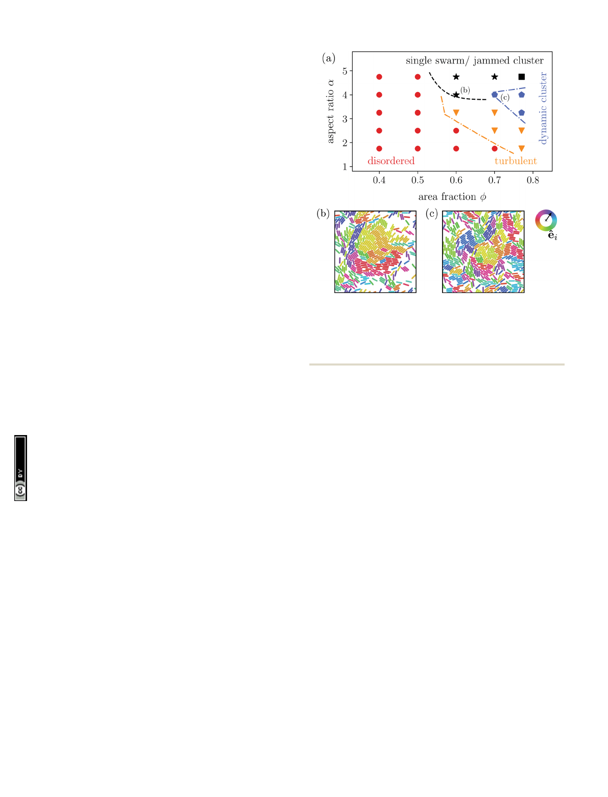
3.3.1 State diagram. For the minimum dipole strength

w=1, i.e., the pusher-type squirmer rods with the largest

force dipole, we study the collective dynamical states as a

function of the aspect ratio aand area fraction f.Acomparison

between the state diagrams of neutral squirmer rods [cf. Fig. 1(c)]

and pusher rods [cf. Fig. 3(a)] already illustrates the strong

influence of the long-ranged hydrodynamic dipole–dipole inter-

actions. Compared to neutral squirmer rods the transition line

from the disordered to other states is shifted to larger area

fractions and new dynamic states arise such as active turbulence

and dynamic clustering. We provide an overview of the observed

dynamic states before presenting a more quantitative analysis in

Section 3.3.2.

Most interestingly, compared to neutral squirmer rods the

flow field of the pusher rod obviously suppresses the formation

of dynamic swarms and impedes the single swarm state, which

only occurs for large aZ4.0. This is in agreement with findings

of Saintillan and Shelley,

who employ slender-body theory to

show that polar and nematic order in systems of elongated

pusher microswimmers is destroyed by their hydrodynamic

flow fields. Likewise, explicit hydrodynamic simulations of

collective dynamics of spherical squirmers show that pushers

create disordered homogeneous systems,

13,109

while pullers

show swarming.

109

An argument for this diﬀerence in the

collective dynamic behavior is found in both implicit

and

explicit

hydrodynamic simulations, which show that pushers

are deflected during collision, while pullers align.

Instead of the suppressed swarming states for ar3.25,

we find a very dynamic or turbulent state. A typical snapshot of

a rod configuration is shown in Fig. 4(a), a video is provided

in the Video 1 (ESI†). Here, the hydrodynamic dipole–dipole

interactions compete with steric interactions that favor the

formation of single swarms at large area fraction fin the case

of neutral rods.

Towards lower fthe turbulent state transi-

tions to the disordered state and towards higher aspect ratio a

to cluster or swarm states.

Similar to other examples of active turbulence in theory and

experiments,

47,49–51,97

we find two cascades in the power spec-

tral density of the squirmer velocities, as we will show in detail

in Section 3.3.2. For the turbulent state at a= 3.25 and f= 0.6

we construct a continuous velocity field v(x,y) to visualize the

turbulent flow pattern and its vortices. A snapshot of the system

and the resulting flow field are shown in Fig. 4(a) and (b),

respectively. We also calculate the vorticity o=(rv)

, which

is shown in Fig. 4(c). To easily obey the periodic boundary

conditions, the vorticity was determined via a Fourier trans-

formation. In all turbulent states, we observe that squirmer

rods show a local alignment, which extends over short streaks,

where squirmer rods swim side by side and head to tail.

However, these streaks buckle and dissolve frequently, leaving

a chaotic pattern of streaks and vortices.

Fig. 3 (a) State diagram of the strongest pusher-type squirmer rods with

w=1 in the parameter space aspect ratio aversus area fraction f.

(b) Snapshot of a single swarm state at a= 4.75 and f= 0.6, (c) snapshot of

a dynamic cluster state at a= 4.0 and f= 0.7 as indicated in the state

diagram. The color of the individual squirmer rods encode their orientation

in the xy-plane.

Soft Matter Paper

Open Access Article. Published on 05 July 2022. Downloaded on 10/27/2022 10:58:01 AM.

This article is licensed under a

Creative Commons Attribution 3.0 Unported Licence.

View Article Online

Loading more pages...