Citation: Ruan, D.; Chen, Y.;
Gühmann, C.; Yan, J.; Li, Z.
Dynamics Modeling of Bearing with
Defect in Modelica and Application
in Direct Transfer Learning from
Simulation to Test Bench for Bearing
Fault Diagnosis. Electronics 2022,11,
622. https://doi.org/10.3390/
electronics11040622
Academic Editors: Martin Sjölund,
Peter Fritzson, Lena Buffoni, Adrian
Pop and Lennart Ochel
Received: 29 January 2022
Accepted: 11 February 2022
Published: 17 February 2022
Publisher’s Note: MDPI stays neutral
with regard to jurisdictional claims in
published maps and institutional affil-
iations.
Copyright: © 2022 by the authors.
Licensee MDPI, Basel, Switzerland.
This article is an open access article
distributed under the terms and
conditions of the Creative Commons
Attribution (CC BY) license (https://
creativecommons.org/licenses/by/
4.0/).
electronics
Article
Dynamics Modeling of Bearing with Defect in Modelica and
Application in Direct Transfer Learning from Simulation to Test
Bench for Bearing Fault Diagnosis
Diwang Ruan 1, Yuxiang Chen 2, Clemens Gühmann 1,* , Jianping Yan 3,* and Zhirou Li 2
1Chair of Electronic Measurement and Diagnostic Technology, Technische Universität Berlin,
2
School of Electrical Engineering and Computer Science, Technische Universität Berlin, 10587 Berlin, Germany;
3School of Vehicle and Mobility, Tsinghua University, Beijing 100084, China
*Correspondence: [email protected] (C.G.); [email protected] (J.Y.)
Abstract:
In data-driven bearing fault diagnosis, sufficient fault data are fundamental for algorithm
training and validation. However, only very few fault measurements can be provided in most
industrial applications, bringing the dynamics model to produce bearing response under defects.
This paper built a Modelica model for the whole bearing test rig, including the test bearing, driving
motor and hydraulic loading system. First, a five degree-of-freedom (5-DoF) model was proposed
for the test bearing to identify the normal bearing dynamics. Next, a fault model was applied to
characterize the defect position, defect size, defect shape and multiple defects. The virtual bearing
test bench was first developed with OpenModelica and then called in Python with OMPython. For
validation of the positive effect of the dynamics model in the direct transfer learning for bearing fault
diagnosis, the simulation data from the Modelica model and experimental data from the Case Western
Reserve University were fed separately or jointly to train a Convolution Neural Network (CNN).
Then the well-trained CNN was transferred directly to achieve the fault diagnosis under the test
set consisting of experiment data. Additionally, 157 features were extracted from both time-domain
and frequency-domain and fed into CNN as input, and then four different validation cases were
designed. The results confirmed the positive effect of simulation data in the CNN transfer learning,
especially when the simulation data were added as auxiliary to experimental data, and improved
CNN classification accuracy. Furthermore, it indicated that the simulation data from the bearing
dynamics model could play a part in the actual experimental measurement when the collected data
were insufficient.
Keywords:
bearing; transfer learning; dynamics model; fault diagnosis; modelica; Convolutional
Neural Network (CNN)
1. Introduction
Bearing fault diagnosis and prognosis can effectively prevent rotating machines from
most failures and therefore have much significance. In recent years, data-driven methods
have gained increasing attention in this field, and many good results have been achieved.
Among the different kinds of data-driven methods, Convolution Neural Network (CNN) is
the most commonly used due to its powerful ability in deep feature extraction and complex
nonlinear mapping. CNN was first introduced to realize bearing fault diagnosis by O.
Janssens in 2016 [
1
]. Thereafter, many improvements and variants have been proposed
to strengthen the CNN’s performance, such as 1D-CNN, 2D-CNN, multiscale CNN and
adaptive CNN [
2
–
5
]. Though satisfying results have been obtained in the extensive re-
search mentioned above, the premise to guarantee such results for data-driven methods is
sufficient data for algorithm training. However, in practice, limited rather than massive
data are typical, which has become a significant barrier of data-driven PHM (Prognostics
Electronics 2022,11, 622. https://doi.org/10.3390/electronics11040622 https://www.mdpi.com/journal/electronics

Electronics 2022,11, 622 2 of 18
and Health Management) being applied in industrial settings. Data augmentation and
generation have been adopted to address this problem. Oversampling was first proposed
for data generation, and the main idea is to generate more samples by direct replication for
such labels that had very few ones [
6
,
7
]. Although this method is simple and efficient to
implement, causes overfitting easily since no new information is incorporated. As another
perspective method for data generation, Generative Adversarial Network (GAN) has al-
ready been used for new sample generation in fault diagnosis, generating new samples
similar to the actual measurement with random noise input. Both W. Zhang and S. Shao
employed GAN to create more vibration data and to expand the available imbalanced
dataset, with results confirming that the diagnosis accuracy could be improved once the
imbalanced data was augmented by GAN [8,9].
This previous research has proven effective in sample generation for small or imbal-
anced datasets. Still, most of these methods are data-driven and generate new samples
merely based on the given existing measurements or random noise, ignoring the physics
mechanism behind data. This brings bearing dynamics model as an alternative to produce
bearing response under given normal and defect conditions. To date, the methods for
bearing dynamics and vibration response simulation can be classified into two categories,
namely, mechanism-based models and signal-based models. Cui et al. proposed a 5-DoF
model to describe bearing’s dynamic behavior [
10
]. Moreover, a defect model was built
to address defect position, defect shape and defect size [
11
]. In terms of bearing response
simulation based on signal analysis, the first model was proposed by McFadden in 1983 to
identify the amplitude spectrum of bearing with a single defect on the inner race [
12
]. In
2000, slight random variations were incorporated into the impulse responses to resemble
actual vibration signals generated by bearing faults [
13
]. After that, Cong et al. put forward
a new fault signal model for bearing with the combination of decaying oscillation fault
signal model and rotor dynamic response influence [
14
]. In a real test bench, dynamics
from driving and loading systems also affect the test bearing response. Nevertheless, to our
exhausted knowledge, nearly all published papers on bearing fault modeling only focus on
the bearing without considering the dynamics from driving motor and loading actuator,
also very limited work has been reported on bearing modeling in Modelica, which defines
the goal to build a whole bearing test bench in this study [
15
]. In this paper, a virtual
bearing test bench is developed in OpenModelica, including test bearing, connecting shaft,
hydraulic loading and force controller, driving motor and speed controller. The test bearing
dynamics model elaborates under normal conditions and various defect scenarios. After
validation, the virtual test bench is used to generate simulation samples. Afterward, the
generated samples are fed into CNN for network training. Finally, the well-trained CNN is
transferred directly to achieve fault diagnosis on pure experiment data collected from the
Case Western Reserve University bearing test rig.
The main innovation of this paper includes: (1) A general platform for bearing dy-
namics simulation and CNN-based fault diagnosis is developed based on OpenModelica
and Python. The calling method and interface are presented, giving a new and efficient
solution for studying the data-driven fault diagnosis with open source languages. (2) The
simulation data from the dynamics model was used for CNN training. In addition, the
positive effect on the CNN’s transfer learning performance from the generated simulation
data was studied and analyzed with four designed validation cases.
This paper’s remaining part is structured as follows: Section 2introduces the modeling
theory of bearing dynamics with defects. Section 3details the implementation process of
the bearing dynamics model in OpenModelica and the calling interface in Python with
OMPython. After that, the feature extraction and fault diagnosis based on CNN are
presented in Section 4. Section 5describes the direct transfer learning of CNN from the
simulation model to the test bench when involved in bearing fault diagnosis and analyzes
the positive effect from simulation data. Finally, Section 6 concludes the whole paper.
Electronics 2022,11, 622 3 of 18
2. Dynamics Modeling of Bearing with Defects
The ball bearing comprises the outer ring, inner ring, cage and rolling elements. A
standard bearing achieves dynamic balance in a stable operating condition, while a series
of impulses will be generated once there is a defect between the contact surfaces. A 5-DoF
dynamics model and a defect model will be introduced in the following.
2.1. The Nonlinear 5-DoF Model
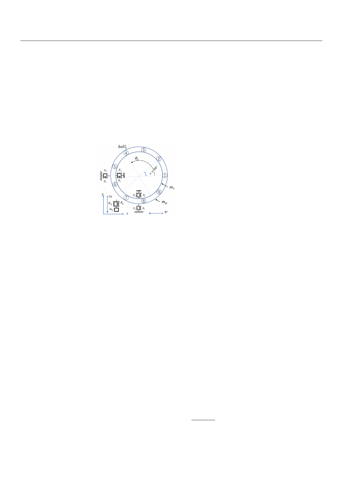
This model describes the nonlinear dynamic behavior of bearing, as shown in
Figure 1.
In the 5-DoF model, 4 DoF represents the horizontal and vertical directions of inner and
outer rings, and 1 DoF stands for the vertical direction of the resonator, which is modeled
as the spring-mass system [10].
Figure 1. The 5-DoF model of bearing [10].
Based on Newton’s second law, the bearing dynamic equilibrium equations can be
formulated as Equation (1) [10].
ms¨
xs+Rs˙
xs+Ksxs+fx=0 ,
ms¨
ys+Rs˙
ys+Ksys+fy=Fy−msg,
mp¨
xp+Rp˙
xp+Kpxp−fx=0 ,
mp¨
yp+ (Rp+RR)˙
yp+ (Kp+Kr)yp−RR˙
yb,
−KRyb−fy=−mpg,
mR¨
yb+RR(˙
yb−˙
yp) + KR(yb−yp) = −mRg.
(1)
fx
and
fy
are contact force at
x
and
y
axis, respectively,
Fy
is external load. The meanings
and values of other variables can be found in [
15
]. According to Hertzian contact theory,
the contact force between rolling element and raceways can be given by:
fj=Kbδ1.5
j, (2)
with
j
from 1 to
nb
,
nb
which represents the number of rolling elements.
Kb
stands for the
ball’s stiffness,
δ
denotes deformation. The deformation of the
j
th ball,
δj
, is determined by
the displacement between the inner and outer races, the angular position
θj
and the total
clearance ccaused by the oil film and assembly clearance, as:
δrawj=xs−xpcos θj+ys−ypsin θj−c. (3)
The angular position of the jth ball can be calculated by Equation (4).
θrawj=2π(j−1)
nb
+ωct+φ0, (4)

Electronics 2022,11, 622 4 of 18
where
φ0
is initial cage angular position and
ωc
is cage angular frequency, which can be
further obtained from shaft frequency ωslike Equation (5).
ωc=1−Db
Dpωs
2, (5)
where Dband Dpare the ball diameter and pitch diameter, respectively.
Usually, there is inevitable sliding for bearings in real applications when a ball rolls
on the raceways. The sliding direction depends on where the ball is located; when the
ball enters the load zone, the angular speed of the ball center is faster than that of the
cage; otherwise, the ball would slide backward. Consequently, with sliding considered, the
angular position of each ball can be modified by Equation (6) [10].
θj=θrawj+ξj1
2randφslip . (6)
There are two constants and a sign function in Equation (6).
φslip
is a parameter
defining the mutation percentage of average contact frequency, which is normally between
0.01 and 0.02 rad.
rand
is a random number with uniform distribution with the range of
[0, 1], and the sign function ξjis expressed as:
ξj=(1, load zone
−1, else (7)
Considering δjshould be nonnegative in physics, its final value is determined by:
δj=Max(δrawj, 0). (8)
With the contact force of each ball obtained from Equation (2), the total contact forces
in xand ydirection are determined with Equations (9) and (10).
fx=
nb
∑
j=1
fjcos θj, (9)
fy=
nb
∑
j=1
fjsin θj. (10)
2.2. Bearing Defect Model
When bearing has defects either on races or balls, an additional deformation,
δf au
,
will be released when the ball moves over the defect zone. Thus, with defect considered,
deformation of the jth ball can be further identified as:
δrawj=xs−xpcos θj+ys−ypsin θj−c−δf auj. (11)
Once bearing deformation under defect is obtained, it can be substituted into
Equations (9) and (10)
. The nonlinear contact force can be calculated and further sub-
stituted into Equation (1) for the fault-bearing response.
δf au
changes with defect position,
defect shape and the number of defects. Due to space limitation, only the modeling of
defect position will be presented in this paper, the modeling of defect size, defect shape,
and multiple defects can be found in the original conference paper [15].
Before defect modeling, four basic geometrical parameters are chosen to feature the
defect, as demonstrated in Figure 2, the defect width
B
, the defect depth
Hd
, the defect
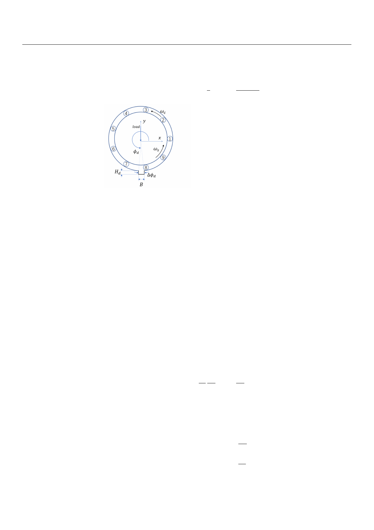
Electronics 2022,11, 622 5 of 18
initial angle
φd
and the defect span angle
∆φd
. Take a defect on the outer ring as an example,
the relation between ∆φdand Bis expressed as:
sin1
2∆φd=B
Db+Dp. (12)
Figure 2. Size definition of defect on the outer ring [15].
Suppose the local defect depth is
cd
, the additional deformation
δf au
generates only
when a ball falls into the defect zone within
φd
and
φd+∆φd
, then the deformation released
by defect on raceway is given by:
δf auj=(cd,φd≤θj≤φd+∆φd
0, else (13)
The defect location on the outer ring or inner ring changes with different rules. For
the outer ring, the defect is fixed at the defect initial angle
φdo
. However, for the inner ring,
the defect location changes with time when the inner ring rotates. Thus,
φd
in Equation (13)
can be further modeled as follows.
φd=(φdo, defect on the outer ring
ωst+φdi, defect on the inner ring (14)
Different from rings, when a defect happens on a rolling element, the defect spins with
ball speed ωband its position φscan be obtained like:
φs=ωbt+φsini , (15)
hereby the ball speed ωbcan be calculated from shaft speed as follows,
ωb=ωs
2
Dp
Db"1−Db
Dpcos α2#. (16)
The defect on balls contacts the inner and outer ring periodically. Besides, the curvature
radii of inner and outer rings are different. Therefore, the same defect span angle
∆φd
produces different angular widths. The angular widths of defect on the outer ring and
inner ring, ∆φbo and ∆φbi, can be calculated by Equations (17) and (18).
∆φbo =∆φd
Db
Do , (17)
∆φbi =∆φd
Db
Di , (18)
with Doand Dias the diameters of outer ring and inner ring, respectively.
Loading more pages...