
Journal of Nonlinear Science (2021) 31:51
https://doi.org/10.1007/s00332-021-09706-4
The Height Invariant of a Four-Parameter Semitoric System
with Two Focus–Focus Singularities
Jaume Alonso1,2 ·Sonja Hohloch2
Received: 28 August 2020 / Accepted: 30 March 2021 / Published online: 19 April 2021
© The Author(s) 2021
Abstract
Semitoricsystemsareaspecialclassofcompletelyintegrablesystemswithtwodegrees
of freedom that have been symplectically classified by Pelayo and V˜uNgo
.c about a
decade ago in terms of five symplectic invariants. If a semitoric system has several
focus–focussingularities,thensomeof these invariantshavemultiplecomponents,one
for each focus–focus singularity. Their computation is not at all evident, especially
in multi-parameter families. In this paper, we consider a four-parameter family of
semitoric systems with two focus–focus singularities. In particular, apart from the
polygon invariant, we compute the so-called height invariant. Moreover, we show
that the two components of this invariant encode the symmetries of the system in an
intricate way.
Keywords Completely integrable Hamiltonian systems ·Semitoric systems ·
Symplectic invariants ·Focus-focus singularities ·Height invariant
Mathematics Subject Classification 37J06 ·37J35 ·37J39 ·53D20 ·70H05 ·70H06
1 Introduction
In the last decades, various efforts have been made towards the construction of
classifications within the theory of completely integrable dynamical systems. These
Communicated by Peter Miller.
BJaume Alonso
Sonja Hohloch
1Technische Universität Berlin, Institute of Mathematics, Str. des 17. Juni 136, 10623 Berlin,
Germany
2Department of Mathematics, University of Antwerp, Middelheimlaan 1, 2020 Antwerp, Belgium
123

51 Page 2 of 32 Journal of Nonlinear Science (2021) 31 :51
classifications are based on invariants that capture various aspects of a system with
respect to different notions of equivalence. They are useful for two main reasons:
they give an overview of all possible systems within a certain class and allow us to
distinguish between non-equivalent systems. If we restrict ourselves to classifications
of symplectic type, important accomplishments are the classification of toric systems,
due to Delzant (1988), Atiyah (1982) and Guillemin and Sternberg (1982) and the
classification of semitoric systems, due to Pelayo and V˜uNgo
.c(2009,2011) and
recently extended by Palmer et al. (2019). Another significant result in this line is the
symplectic classification of completely integrable systems using characteristic classes,
introduced by Zung (2003).
Semitoric systems are a class of dynamical systems defined on connected four-
dimensionalsymplecticmanifolds, introduced by V˜uNgo
.c(2007).Theyareintegrable
systems, so they have two conserved quantities, one of which is a proper map that
induces an effective circle action. Moreover, all singularities are required to be non-
degenerate and must not have hyperbolic components. From a topological point of
view,thesesystemscanbedescribedusingthetheoryofsingularLagrangianfibrations,
cf. Byrd and Friedman (1954). The original definition by V˜uNgo
.c(2007) allowed for
a diffeomorphism on the base, but it was later adapted by Pelayo and V˜uNgo
.c(2009)
for classification purposes, removing this diffeomorphism.
From the symplectic point of view, one of the motivations to study semitoric sys-
tems comes from the analysis of systems with monodromy in the quantum physics
and chemistry literature, see, for example, Child et al. (1999), Sadovskii and Zhilin-
skii (1999) for a theoretical approach and Assémat et al. (2010), Fitch et al. (2009),
Winnewisser et al. (2005) for experimental studies.
In this setting, one has the joint spectrum of a set of unknown quantum operators
and wants to recover information about the system. An overview of the possible can-
didate systems can be obtained by means of a classification. Since classical systems
are generally easier to understand, one can make use of Bohr’s correspondence prin-
ciple or Zauberstab and focus on constructing a classification for classical systems.
However, in order for the results to be valid after quantisation, it is important that this
classification preserves the symplectic structure, cf. Pelayo (2021) for more details on
this approach.
Two foundational examples of the semitoric systems theory are the coupled spin-
oscillator and the coupled angular momenta. The first one is a particular case of
the Jaynes and Cummings (1963) model from quantum optics and it consists of the
coupling of a classical spin on the two-sphere S2with a harmonic oscillator on the
plane R2, cf. Pelayo and V˜uNgo
.c(2012). The second one is the classical version of
the addition of two quantum angular momenta, defined on the product of two copies
of S2. It models, for example, the reduced Hamiltonian of a hydrogen-like atom in the
presence of parallel electric and magnetic fields, cf. Sadovskii et al. (1996). In the last
years, several other examples of semitoric systems have been discovered: Hohloch
and Palmer (2018) introduced a family with two focus–focus points, Le Floch and
Palmer (2018) proved the existence of examples in all Hirzebruch surfaces and De
Meulenaere and Hohloch (2021) proposed a system with four focus–focus points that
has double pinched focus–focus fibres for a certain value of the parameter.
123

Journal of Nonlinear Science (2021) 31 :51 Page 3 of 32 51
The classification of semitoric systems is based on five symplectic invariants: the
number of focus–focus points, the polygon invariant, the height invariant, the Taylor
series invariant and the twisting index invariant.
The survey article by Alonso and Hohloch (2019) gives an overview of the state
of the art concerning examples and computations of invariants reached in 2019. Note
that the computation of these invariants is far from trivial, especially if the aim is to
make a general calculation of the invariants for a whole family of systems depending
on several parameters, instead of for only one explicitly given, concrete system.
So far, the full list of invariants has only been computed for the two foundational
examples. The computation of the invariants in these two cases is based on the use of
the properties of elliptic integrals, cf. Alonso (2019). In the case of the coupled spin-
oscillator, it was initiated by Pelayo and V˜uNgo
.c(2012) and completed by Alonso
et al. (2019). In this case, two parameters are taken into account, but the dependence
is quite simple. For the coupled angular momenta, it was initiated by Le Floch and
Pelayo (2018) and completed by Alonso et al. (2020). In this case, the dependence is
of three parameters and significantly more involved.
Expressing the invariants as a function of the parameters of the system is important
because, besides the quantitative results, it also allows for qualitative considerations.
For instance, one can compare the roles played by geometric parameters, i.e. those
related to the symplectic manifold, and by coupling parameters, i.e. those only appear-
inginthemomentummap.Incase some parameters also affectthe type of singularities,
for example making focus–focus singularities appear and disappear, one can also see
what happens to the invariants as the critical values of the parameters are approached.
Inbothfoundationalexamples,the invariantsdisplaythesymmetriesofthesystems.
Moreover, for the coupled angular momenta, the terms of the Taylor series invariant
go to infinity as the coupling parameter approaches the critical values, cf. Alonso
et al. (2020). However, a limitation of these examples is that the number of focus–
focus points is at most one. Semitoric systems with more than one focus–focus point
are interesting because, in this case, the symplectic invariants have multiple compo-
nents, one for each focus–focus point. So the different components can (and should)
be compared with each other. In particular, it is interesting to see how the different
components depend on the parameters of the system and how they reflect the possible
symmetries of the system.
Notethatthepresenceofmultiplefocus–focuspointsincreasesthecomplexityofthe
computations significantly. So far, the only results in this direction are the computation
of the polygon invariant and the height invariant of two families of systems with a
relativelysimpledependenceontwoparameters,cf.LeFlochandPalmer(2018).There
is, in general, a certain trade-off between, on the one hand, the qualitative richness of
having the invariants expressed as functions of several parameters and, on the other
hand, the feasibility of their computations.
In the present paper, we choose the former option, i.e. focusing on dependence
on multiple parameters. We managed to compute the number of focus–focus points
invariant, the polygon invariant, and the height invariant. However, due to the number
of parameters and the complexity of the computations, the Taylor series invariant and
the twisting index invariant are beyond current computational methods and resources,
cf. Alonso (2019).
123

51 Page 4 of 32 Journal of Nonlinear Science (2021) 31 :51
Let (M,ω)be the symplectic manifold M=S2×S2with symplectic form ω=
−(R1ωS2⊕R2ωS2), where ωS2is the standard symplectic form of the unit sphere and
0<R1<R2or 0 <R2<R1.Given(x1,y1,z1,x2,y2,z2)Cartesian coordinates
in Mand s1,s2∈[0,1], we consider the integrable system (M,ω,F), where F:=
(L,H)is defined by
⎧
⎪
⎨
⎪
⎩
L(x1,y1,z1,x2,y2,z2):= R1z1+R2z2,
H(x1,y1,z1,x2,y2,z2):= (1−2s1)(1−s2)z1+(1−2s1)s2z2
+2(s1+s2−s12−s22)(x1x2+y1y2).
(1)
It is a family of semitoric systems that can have up to two focus–focus singularities
and depends on four parameters in total, two geometric parameters R1,R2>0,
R1= R2and two coupling parameters s1,s2∈[0,1].
Our first result is the computation of the number nFF of focus–focus singularities,
which is the first symplectic invariant of a semitoric system:
Theorem 1 The number of focus–focus points invariant of system (1)is nFF =0if
E>0and nFF =2if E <0, where
E=R22(1−2s1)2(−1+s2)2+R12(1−2s1)2s22−2R1R2(8(−1+s1)2s12
+s2−12(−1+s1)s1s2+(7+12(−1+s1)s1)s22−16s23+8s24).
If E =0, the system fails to be semitoric.
Theorem 1is a reformulation of Theorem 15 and Corollary 16 stated later in the
paper. The number of focus–focus points invariant is illustrated in Fig. 6. The image
of the momentum map of system (1) is plotted in Fig. 5which is the starting point
for the computation of the polygon invariant. The polygon invariant is the result of a
straightening procedure of the image of the momentum map, introduced in V˜uNgo
.c
(2007), as a generalisation of Delzant’s polygon invariant for toric systems, cf.Delzant
(1988).
Theorem 2 The polygon invariant of the system (4)is determined by the following
cases:
•If nFF =2, the polygon invariant is the ((Z2)2×Z)-orbit generated by any of the
polygons represented in Fig. 7.
•If nFF =0and (s1,s2)lies in the same connected component as the point (0,0)
or (1,1), then the polygon invariant is the Z-orbit generated by the polygon in
Fig. 7b.
•If nFF =0and (s1,s2)lies in the same connected component as the point (1,0)
or (0,1), then the polygon invariant is the Z-orbit generated by the polygon in
Fig. 7c.
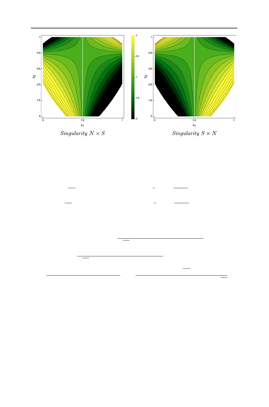
Whenever nFF =2, the height invariant is defined and has two components. This
invariant describes the position of the focus–focus values in the polygon after the
straightening procedure. Their explicit computation is our main result:
123
Journal of Nonlinear Science (2021) 31 :51 Page 5 of 32 51
(b)(a)
Fig. 1 Representation of the height invariant for R1=1, R2=4
Theorem 3 For the values of (s1,s2)for which the system (1)has two focus–focus
singularities, the height invariant h := (h1,h2)is given by
h1=−1
2πF(s1,s2,R1,R2)+2u(s1−1
2)(s2−R2
R2+R1),
h2=1
2πF(s1,s2,R1,R2)+2u−(s1−1
2)(s2−R2
R2+R1)=2−h1
where u is the Heaviside step function and
F(s1,s2,R1,R2):= 2R2arctan γC
√γA(2s1−1)(R2(s2−1)+R1s2)
+2R1arctan γD
√γA(2s1−1)(R2(s2−1)+R1s2)
+(2s1−1)(R2(s2−1)+R1s2)
2s12−s1+s22−s2log −√γB
2(R2+R1)s12−s1+s22−s2+√γA.
The height invariant is plotted in Fig. 1and the coefficients γAγB,γCand γDare
explicitly stated in Proposition 4.
Thecoefficientsencodethedependenceoftheheightinvariantonthevariousparam-
eters. This dependence is polynomial, except for some radicals.
Proposition 4 The coefficients γAγB,γCand γDof Theorem 3are given by
γA:= −R22(1−2s1)2(s2−1)2+2R2R18s14−16s13+4s123s22−3s2+2
−12s1(s2−1)s2+s28s23−16s22+7s2+1−R12(1−2s1)2s22
123
Loading more pages...