A Fractional Time-Derivative Model for Severe Wear: Hypothesis and Implications [original]

A Fractional Time-Derivative Model for

Severe Wear: Hypothesis and

Implications

Ivan Argatov*

Institut für Mechanik, Technische Universität Berlin, Berlin, Germany

Based on the example of wear of polymers, which exhibit a power-law time variation of the

wear loss under constant loading conditions, a fractional time-derivative wear equation has

been introduced. The wear contact problem with a ﬁxed contact zone is solved using the

known method of separation of spatial and time variables. It is shown that during the wear

process, the contact pressure approaches a uniform distribution over the contact area,

which is termed as a quasi-steady-state solution, since the mean volumetric wear rate

does not tend to become constant. It is of interest that the contact pressure variation

displays a decaying oscillatory nature in the case of severe wear, when the mean

volumetric wear rate increases with time.

Keywords: severe wear, fractional time derivative, wearing-in, quasi-steady state, wear equation

1 INTRODUCTION

Wear is a tribological phenomenon that accompanies contact interaction of solids with interfacial

sliding between their surfaces and manifests itself primarily in gradual loss of material due to the

subsurface damage accumulation and surface degradation (Zmitrowicz, 2006). In wear material

testing, the wear loss is usually measured in terms of the volume of lost material, V, which yields the

wear depth, w, by relating to the area of contact, A,as

wV

A.(1)

Eq. 1 tentatively assumes that the wear loss is the same at each point of the contact zone, and this

condition is characteristic of the steady-state wear process (Dundurs and Comninou, 1980;Páczelt

and Mróz, 2007).

Usually, sliding wear tests are performed under constant normal loading conditions, which are

characterized by either contact load, P, or mean contact pressure,



pP

A.(2)

In the cases of mild or moderate wear, after some initial running-in (Wright and Kukureka, 2001;

Khonsari et al., 2021) or wearing-in (Blau, 2005) period of time, the condition of steady state

p(x, t)≡

pis realized at the contact interface and maintained for a long time period, during which

the wear material characteristics have been measured.

In the steady-state wear process, the linear wear rate, deﬁned as the time derivative _

wdw/dt,is

constant in time, and moreover, the contact pressure pachieves a constant value over the entire

contact zone. So, in the steady-state wear regime, the volumetric wear loss Vwill be a linear function

of the time variable t, and thus, the linear wear rate can be evaluated as

Edited by:

Yu Tian,

Tsinghua University, China

Reviewed by:

Emanuel Willert,

Technical University of Berlin,

Germany

Feodor M Borodich,

Cardiff University, United Kingdom

*Correspondence:

Ivan Argatov

[email protected]erlin.de

Specialty section:

This article was submitted to

Tribology,

a section of the journal

Frontiers in Mechanical Engineering

Received: 26 March 2022

Accepted: 08 April 2022

Published: 27 April 2022

Citation:

Argatov I (2022) A Fractional Time-

Derivative Model for Severe Wear:

Hypothesis and Implications.

Front. Mech. Eng 8:905026.

doi: 10.3389/fmech.2022.905026

Frontiers in Mechanical Engineering | www.frontiersin.org April 2022 | Volume 8 | Article 9050261

ORIGINAL RESEARCH

published: 27 April 2022

doi: 10.3389/fmech.2022.905026

wVt

()

−Vt

()

2−t1

()

,(3)

where t

and t

are any two different moments of time taken

during the steady-state period.

In many cases, the wear equation can be written in the

following form (Kragelsky, 1965):

VkwPvt.(4)

Here, vis the sliding velocity, and k

is the wear coefﬁcient. In

view of Eqs 1,2,Eq. 4 can be represented as

wkw

pv, (5)

which is known as Archard’s equation (Meng and Ludema, 1995),

though similar wear equations were introduced earlier by Reye

(1860),Khrushchov and Babichev (1941), and Holm (1946). The

wear coefﬁcient k

is determined during the steady-state

conditions by using Eqs 3,5.

A generalization of the wear Eq. 4, which was suggested by

Rhee (1970) for polymer-bonded friction materials, takes the

form

VKwPγvβtα,(6)

where K

is the wear factor, and α,β,γare parameters. However,

while Eq. 6 has been successfully used to predict the wear

resistance of polymer composite materials designed for

extreme environmental conditions (Gardos, 1982;Sedakova

and Kozyrev, 2021), there is a problem with applying the wear

Eq. 6 for solving the wear contact problems with the spatial-

temporal variation of the contact pressures (Grzelczyk and

Awrejcewicz, 2015;Ciavarella et al., 2020).

In recent years, there has been a growing interest in modeling

severe wear (Nguyen et al., 2018;Popov and Pohrt, 2018;Li et al.,

2020). In a broad sense, severe wear is deﬁned as a form of wear

characterized by a rapid increase in the amount and size of wear

particles (Blau, 1992). In many situations, the regime of severe

wear can be characterized by the absence of any steady-state

regime under constant conditions. This is so, for example, in wear

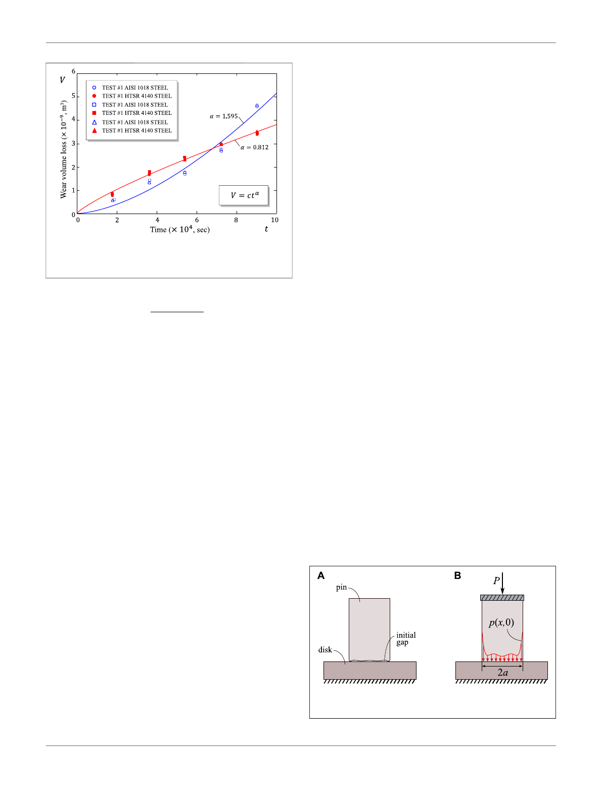
of polymers (Viswanath and Bellow, 1995), when under constant

normal load and sliding speed (see Figure 1), the wear volume

loss Vvaries proportionally to some power of time, that is t

, and

therefore, the wear rate _

wwill be a function of time (proportional

to t

α−1

) during the entire testing period.

It is clear that in experiments like that, whose results are shown

in Figure 1,Eq. 3 is not applicable. Instead we can consider the

ratio V(t)/tthat deﬁnes the mean volumetric wear rate. The two

cases α= 0.812 and α= 1.595 differ by the decreasing/increasing

trend of this quantity. The wear process with increasing in time

mean volumetric wear rate (that is when α>1) will be termed as

severe wear in a narrow sense. At the same time, the case α<1

may called mild wear, as the wear rate decreases towards zero

during the wear process.

Further, when comparing the Archard Eq. 4 with the Rhee Eq.

6, we see that for polymers the Archard wear coefﬁcient k

, which

is evaluated as the ratio V/Pvt, is found to depend on time, that is

kw~tα−1. This means that for polymer-bonded friction

materials, for which the Rhee wear equation applies, the

concept of wear coefﬁcient as a constant characteristic of

tribo-pair is not applicable. However, the two cases α<1 and

α>1 drastically differ in the time variation of the linear wear rate.

In what follows, to avoid misinterpretations of mild and severe

wear regimes, these two cases will be termed as the sub-Archard

and super-Archard regimes of wear.

However, a natural concern arises about the effect of the

wearing-in period, when the initial contact pressure evolves

due to the contact geometry adaptation (Argatov I and Chai,

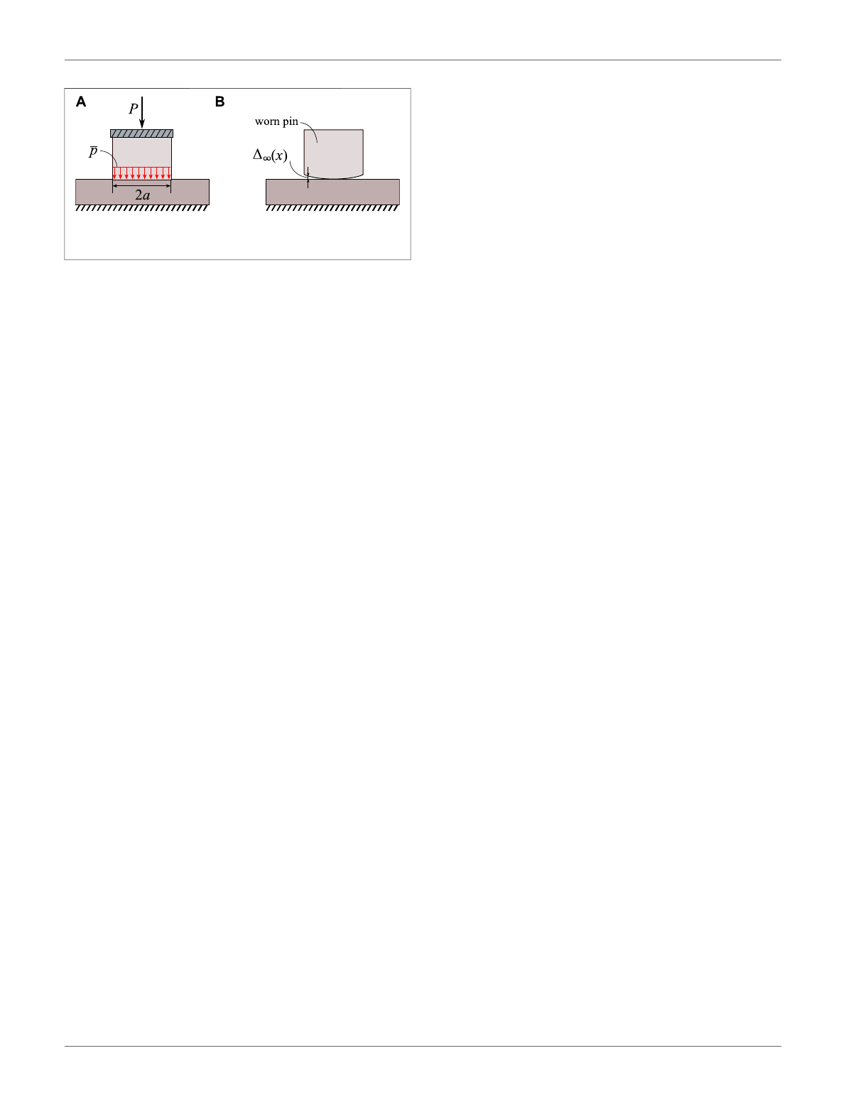
2020). In a pin-on-disk sliding wear tests, when a wearable pin is

put on an abrasive disk, there exists a small initial gap between the

surfaces brought into contact (see Figure 2A), which inﬂuences

the initial contact pressure, p(x,t)att= 0, in the loaded state (see

Figure 2B).

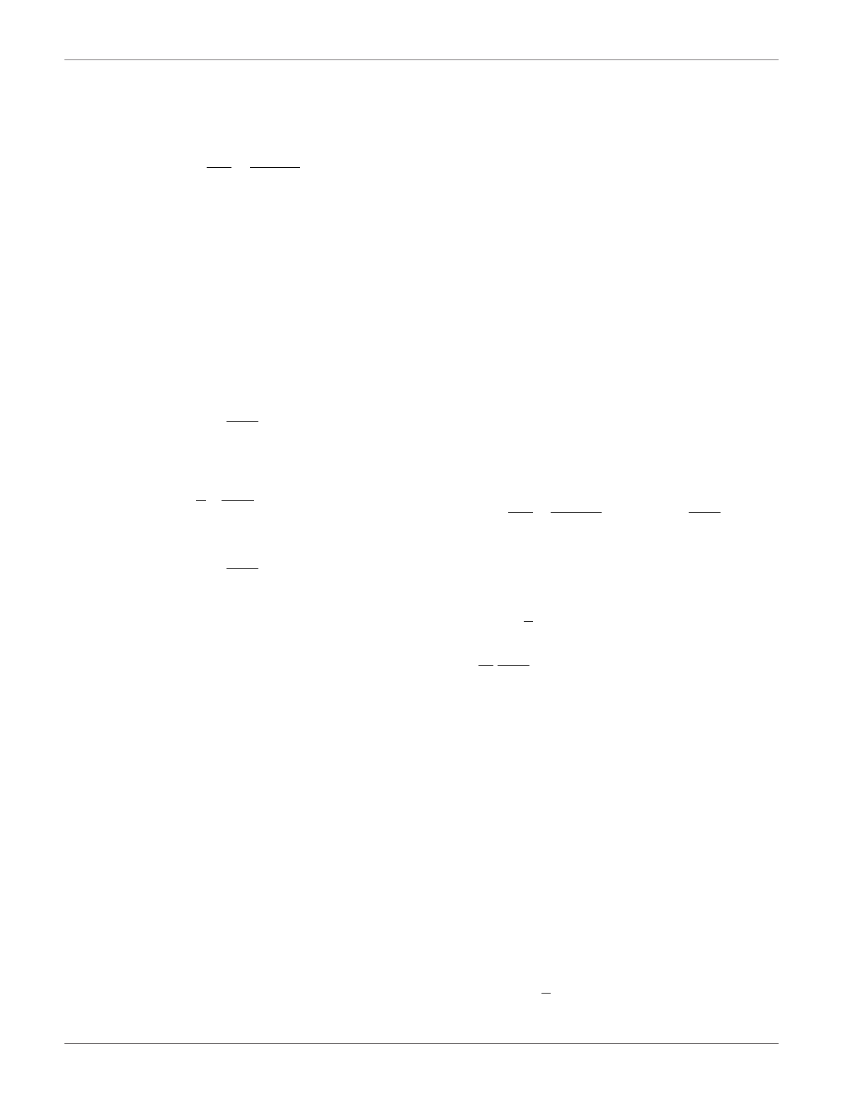
During the wear process, because of the contact geometry

adaptation, the contact pressure p(x,t) evolves in time and

approaches a steady-state pattern of uniform distribution over

the contact zone (see Figure 3A). The corresponding steady-state

shape of the pin surface facing the disk is characterized by the

limiting gap function, Δ

∞

(x), which does not depend on the initial

gap (see Figure 3B).

FIGURE 1 | Volume loss vs. time on linear coordinates with best ﬁt

power-law lines for Delrin against two counterparts (based on the

experimental data taken obtained by Viswanath and Bellow (1995)).

FIGURE 2 | Initial contact conﬁguration: (A) Unloaded state; (B)

Loaded state.

Frontiers in Mechanical Engineering | www.frontiersin.org April 2022 | Volume 8 | Article 9050262

Argatov A Fractional Time-Derivative Model

When the theoretical modeling framework of the contact

geometry adaptation (Figures 2,3) is applied to the case of

super-Archard wear, the main problem to solve in this way is a

generalization of the experimentally observed non-stationary

relation between _

wand 

pconst for the practically important

case p≠const. To date there are no publications on

generalizations of the Rhee model (6) similar to the Archard

wear equation, which follows from Eq. 5 by replacing the mean

contact pressure 

pwith the contact pressure p. It should be

stressed that the same approach does not work for the Rhee wear

Eq. 6. To this extent, the concept of fractional time-derivative can

be efﬁciently applied to gain insight into the contact pressure

evolution in severe wear.

In recent years, the apparatus of fractional differentiation

has been used in mechanics, in particular, to generalize models

of diffusion (Mainardi, 1996), rough contact (Argatov, 2003),

and viscoelasticity (Su et al., 2021). In the present study, we use

the classical Riemann–Liouville derivative. It should be noted

that a number of different approaches exist to introduce a

more general notion of the derivative (Ortigueira and

Machado, 2015). In particular, a so-called fractal fractional

derivative (Chen et al., 2010;He, 2011) does not involve the

integral convolution and represents a local operator. However,

whereas fractals have emerged as a useful mathematical tool in

tribological research (Ling, 1990;Borodich and Onishchenko,

1993;Borodich, 1999), the present study pioneers the use of

concept of the fractional derivative in modeling wear

processes.

Since the theory of wear contact problem is well established

(Aleksandrov and Kovalenko, 1980;Kovalenko, 1985), we adopt

the approach suggested in the constructive review (Argatov I and

Chai Y. S, 2020) and take a general point of view on the

description of the pin/disk contact interaction, which is

applicable both in the three- and two-dimensional settings. To

illustrate the contact pressure evolution, we consider a two-

dimensional wear contact problem (Galin, 1976), for which a

detailed analysis has been available in the literature (Aleksandrov

et al., 1978;Argatov and Fadin, 2011). It is anticipated that with

certain modiﬁcations the fractional time-derivative approach

developed below can be applied to model other temporary-

spatial severe damage processes like mechanochemical

corrosion (Sedova and Pronina, 2022), wear/scratch damage

(Dasari et al., 2009), and wear of metamaterials (Garland

et al., 2020).

The rest of the paper is organized as follows. In Section 2,we

introduce a fractional time-derivative(FTD)wearequationasa

straightforward generalization of the Archard wear equation by

replacing the time derivative in the deﬁnition of the linear wear

rate with appropriate fractional derivative. The FTD wear

equation when applied under constant load conditions

predicts a power-law time variation for the volumetric wear

similar to the Rhee wear equation. This observation explains the

main goal of the present study and that is to generalize the Rhee

wear equation to the case of non-constant (spatial-temporal)

variations of the contact pressure. It is hypothesized that the

FTD wear equation provides such a generalization. The main

body of the paper is devoted to the analysis of implications

drawn from the solution of the model wear contact problem

formulated in Section 3. In particular, the existence of a quasi-

steady state is identiﬁed in Section 4 and, using the method of

variables separation (Section 5), the evaluation of the contact

pressure towards the quasi-steady state is considered in detail in

Section 6.Aparticularlynovelaspect—oscillatory nature—of

the contact pressure variations is discussed in Section 7.The

spatial-temporal variation of the worn proﬁle is presented in

Section 8.Finally,inSection 9, we discuss the obtained results

and further generalizations and formulate the conclusions.

2 FRACTIONAL TIME-DERIVATIVE WEAR

EQUATION

In its basic version due to Archard (1953), the wear equation

linearly relates the wear rate at a point with coordinate xand at

time tto the contact pressure as

wx,t

()

κpx,t

() (7)

with some constant κ, which is related to the wear coefﬁcient, k

as κ=k

v, where vis the speed of relative sliding at the contact

interface.

Under the assumption that the worn material is absent at the

initial moment t= 0 , that is w(x,0)=0,Eq. 7 is equivalent to the

relation

wx,t

()

κ

px,τ

()

dτ.(8)

The integral form Eq. 8 of the wear Eq. 7 is used in

formulating the wear contact problems (Galin, 1976;Argatov

and Tato, 2012), as the wear depth w(x,t) directly describes the

evolution of the contact geometry in the direction normal to the

contact interface.

Let us replace the differentiation with respect to time on the

left-hand side of Eq. 7 with a more general notion of the

derivative. In particular, we make use of the fractional

Riemann–Liouville derivative of order α, which will be

denoted by Dα

t. In this way, we straightforwardly arrive at the

equation

Dα

twx,t

()

κpx,t

()

,(9)

FIGURE 3 | Steady-state contact conﬁguration: (A) Loaded state; (B)

Unloaded state.

Frontiers in Mechanical Engineering | www.frontiersin.org April 2022 | Volume 8 | Article 9050263

Argatov A Fractional Time-Derivative Model

which contains two parameters, namely, κand α.

In the framework of fractional calculus, from Eq. 9, it follows

that

wx,t

()

κ

Γα

()



px,τ

()

t−τ

()

1−αdτ,(10)

where Γ(x) is the gamma function.

The right-hand side of Eq. 10 contains the Riemann–Liouville

integral of order αwhich is consistent with the inversion of the

respective fractional derivative appearing in Eq. 9.

It is to emphasize that by taking α=1inEq. 10, in view of the

normalization condition Γ(1) = 1, we recover the integral form

Eq. 8 of the non-fractional Archard wear equation. Therefore, it

makes sense to assume that 0 <α<2, since Eq. 9 generalizes

Archard’sEq. 7, which exactly corresponds to the basic case α=1.

Remark 1. Observe that in the case of steady state, when

p(x, t)≡

p,Eq. 10 yields

wκ

αΓα

()

tα,(11)

and thus, the mean linear wear rate (evaluated from the very onset

of the wear process) will be non-constant

tκ

αΓα

()

tα−1.

In view of Eq. 1, from Eq. 11, it follows that

VκP

αΓα

()

tα. (12)

Eq. 12 can be ﬁtted to the experimental data shown in Figure 1

to uniquely determine both parameters κand α.

3 WEAR CONTACT PROBLEM

FORMULATION

Following Komogortsev (1985) and Argatov and Fadin (2011),

we consider a wear contact problem for an elastic solid (pin) in

contact with a rigid base (disk) with a ﬁxed zone of contact, x∈ω,

under a constant normal load, P. In this case, the resultant of the

contact pressure p(x,t) satisﬁes the equilibrium equation



px,t

()

dxP, t ≥0. (13)

The wear contact problem can be reduced to the following

governing integral equation in the domain x∈ω,t≥0, which

involves two unknowns, namely, the contact pressure p(x,t) and

the contact displacement δ

(t):



Kx,ξ

()

pξ,t

()

dξδ0t

()−Δ0x

()

+wx,t

()[]

. (14)

Here, K(x,ξ) is a given surface-inﬂuence function (with xand ξ

being the points of observation and integration), Δ

(x) is a known

function of initial gap between the contacting surfaces, and w(x,t)

is the wear depth which is related to the contact pressure p(x,t)by

Eq. 10. It is to note that the gap function is usually subject to the

centering condition Δ

(0) = 0.

We recall that the surface-inﬂuence function K(x,ξ)isdeﬁned

as the normal component of the corresponding vector Green’s

function restricted to the surface of the elastic solid, and thus, the

equilibrium equations inside the elastic solid (Shillor et al., 2004)

are naturally satisﬁed by the construction of the function K(x,ξ).

The reduction of the wear contact problem to the corresponding

governing integral equation is well known (Argatov I and Chai Y.

S, 2020) and allows applying the boundary element method

(Sfantos and Aliabadi, 2006) for the direct evaluation of the

contact pressures.

4 UNIFORM CONTACT PRESSURE AS A

QUASI-STEADY STATE

By integrating Eq. 10 over the contact interval and taking into

account the equilibrium Eq. 13, we derive the following the

relations for the volumetric wear loss:

()

wx,t

()

κ

Γα

()



dτ

t−τ

()

1−α

px,τ

()

dxκPtα

αΓα

()

(15)

Thus, making use of Eq. 15 and following the previously

introduced method (Komogortsev, 1985), we can reduce the

governing integral Eq. 14 to the equation



Kx,ξ

()

−1

AK1ξ

()

pξ,t

()

−pξ,0

()

dξ+wx,t

()

κP

tα

αΓα

()

,(16)

where x∈ωand t>0. Moreover, Adenotes the measure of the

contact area deﬁned as

A

dx, (17)

and we have introduced the notation

K1ξ

()



Kx,ξ

()

dx. (18)

The form of Eq. 16 is preferable in wear contact problems

(Komogortsev, 1985), as the effect of the initial contact

conﬁguration, which is associated with the gap function Δ

(x), is

now incorporated into the initial contact pressure density p(x,0).

Now, let us introduce the notation for the mean contact

pressure and the point-wise deviation of the contact pressure

from its mean value



pP

A, q x, t

()

px,t

()

−

p. (19)

Frontiers in Mechanical Engineering | www.frontiersin.org April 2022 | Volume 8 | Article 9050264

Argatov A Fractional Time-Derivative Model

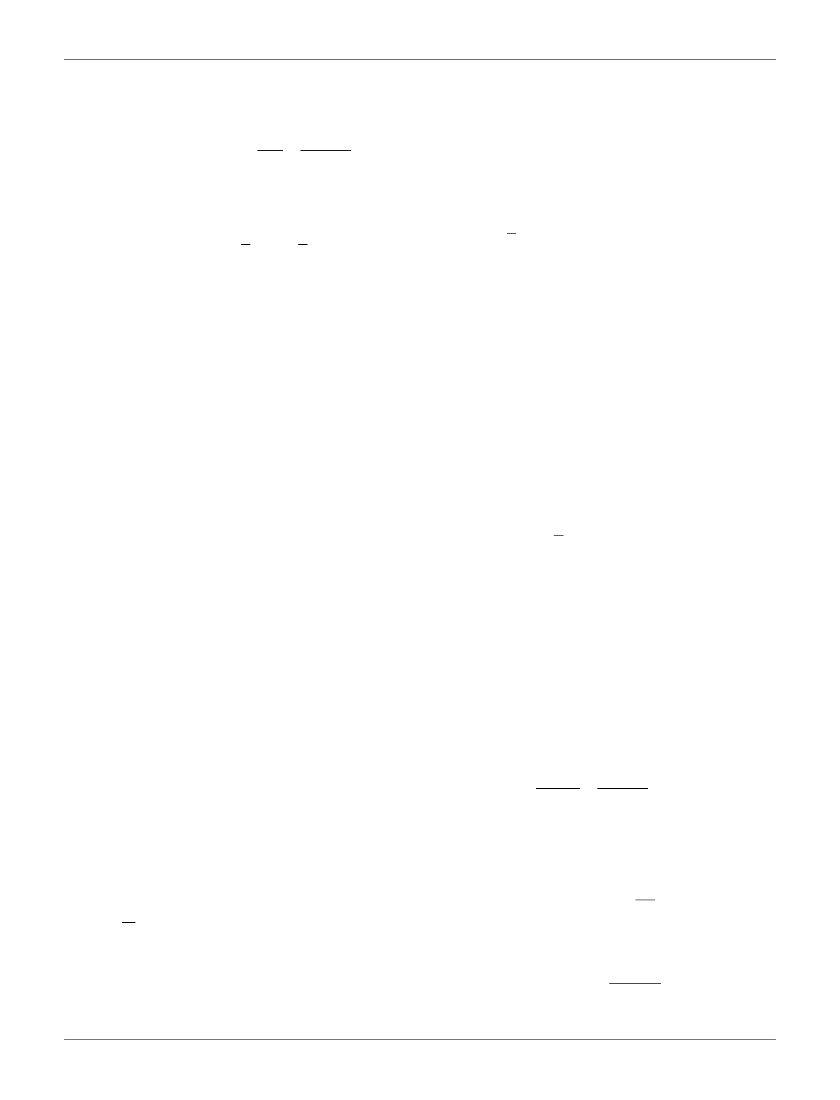
Thus, in view of (Eqs 15,19), Eq. 16 can be rewritten in the

form



K2x, ξ

()

qξ,t

()

−qξ,0

()

dξ+κ

Γα

()



qx,τ

()

t−τ

()

1−αdτ0,

(20)

where x∈ωand t>0, and we have introduced the notation

K2x, ξ

()

Kx,ξ

()

−1

AK1ξ

()

−1

AK1x

()

. (21)

We note that in regard to the kernel of the integral Eq. 16, the

third term on the right-hand side of Eq. 21 has been introduced

for symmetrization (Argatov and Chai, 2019). This is convenient

but does not affect the result because of the zero-mean property



qξ,t

()

dξ0,t≥0,(22)

which follows from the deﬁnition (19)

of the function q(x,t) and

the equation of equilibrium Eq. 13.

To this end, the behavior of the residual function q(x,t) as time

progresses is shown to be described by Eq. 20. By analogy with the

wear contact problems based on the Archard wear equation, it

can be anticipated that the deviation of the contact pressure from

its mean value diminishes with time. In the case under

consideration, we also ﬁnd that q(x,t)→0ast→∞, and

hence the mean contact pressure 

pwill be termed as a quasi-

steady-state solution.

5 NON-DIMENSIONALIZATION AND

SEPARATION OF VARIABLES

For the sake of simplicity, we assume that the pin material is

isotropic and can be characterized by Young’s modulus, E, and

Poisson’s ratio, ]. In contact mechanics, an important role is

played by the reduced elastic modulus E*=E/(1 −]

). Also, let a

denote a characteristic size of the contact domain ω, which can be

taken to be equal to the half-diameter of ω.

Following Komogortsev (1985), we take advantage of the fact

that Eq. 20, in view of Eq. 10, is in a separable form (the kernel

function K

(x,ξ) does not depend on the time variable t) that

makes it possible to construct its solution in the form

qx,t

()



∞

n1

bnt

()

ϕnx

()

,(23)

where ϕ

(x) is the nth eigenfunction of the integral operator with

the kernel K

(x,ξ) given by Eq. 21, i.e.,

a

K2x, ξ

()

ϕnξ

()

dξλnϕnx

()

,x∈ω. (24)

We note that the non-dimensionalising factor E*/ahas been

introduced on the left-hand side of Eq. 24 to ensure that the

eigenvalues λ

,λ

,... are dimensionless. It is pertinent to note

here that, in view of Eqs 21,22, the eigenfunctions possess the

zero-mean property



ϕnξ

()

dξ0n1,2,...

()

. (25)

Without loss of generality, we assume that the solutions of the

eigenvalue problem Eq. 24 are normalized as

A

ϕnξ

()

2dξ1n1,2,...

()

. (26)

Thus, taking into account relations (19)

and Eq. 23, we can

represent the contact pressure in the form

px,t

()



p+

∞

n1

bnt

()

ϕnx

()

,(27)

where 

pis given by (19)

, and the set of coordinate functions

(x) is uniquely deﬁned by Eqs 24,26).

By setting t= 0, from Eq. 27, it follows that

px,0

()



p+

∞

n1

bn0

()

ϕnx

()

,(28)

where p(x, 0) solves the integral equation of initial contact, which

is obtained from Eq. 14 by setting t= 0, whereas, in view of Eq. 26,

the coefﬁcients of the inﬁnite sum are given by

bn0

()

1

A

px,0

()

−



ϕnx

()

dx. (29)

In the next section, we consider the evolution of the functions

(t), which satisfy the initial conditions (29). The corresponding

equation is simply obtained by substituting the expansion (Eq.

23) into Eq. 20 and utilizing Eq. 24.

6 EVOLUTION OF THE CONTACT

PRESSURE TOWARDS THE

QUASI-STEADY STATE

In view of Eq. 24, the series solution Eq. 23 satisﬁes Eq. 20, if and

only if

bnt

()+E*κ

λnaΓα

()



bnτ

()

t−τ

()

1−αdτbn0

()

. (30)

Equation 30 is classiﬁed as Abel’s integral equation of the

second kind (see, e.g., (Gorenﬂo and Mainardi, 1997;Gorenﬂo

et al., 2014)), and its solution b

(t) is given in the form

bnt

()bn0

()

Eα−E*κ

λnatα

 (31)

in terms of the single-parameter Mittag-Lefﬂer function of order

α,deﬁned as

Eαx

()



∞

k0

Γαk+1

()

,(32)

Frontiers in Mechanical Engineering | www.frontiersin.org April 2022 | Volume 8 | Article 9050265

Argatov A Fractional Time-Derivative Model

Loading more pages...