
International Journal of Computer Assisted Radiology and Surgery (2021) 16:2089–2097
https://doi.org/10.1007/s11548-021-02482-2
ORIGINAL ARTICLE
Detecting failure modes in image reconstructions with interval neural
network uncertainty
Luis Oala1·Cosmas Heiß2·Jan Macdonald2·Maximilian März1·Gitta Kutyniok3·Wojciech Samek1
Received: 8 April 2021 / Accepted: 10 August 2021 / Published online: 4 September 2021
© The Author(s) 2021
Abstract
Purpose The quantitative detection of failure modes is important for making deep neural networks reliable and usable
at scale. We consider three examples for common failure modes in image reconstruction and demonstrate the potential of
uncertainty quantification as a fine-grained alarm system.
Methods We propose a deterministic, modular and lightweight approach called Interval Neural Network (INN) that produces
fast and easy to interpret uncertainty scores for deep neural networks. Importantly, INNs can be constructed post hoc for
already trained prediction networks. We compare it against state-of-the-art baseline methods (MCDrop,ProbOut).
Results We demonstrate on controlled, synthetic inverse problems the capacity of INNs to capture uncertainty due to noise
as well as directional error information. On a real-world inverse problem with human CT scans, we can show that INNs
produce uncertainty scores which improve the detection of all considered failure modes compared to the baseline methods.
Conclusion Interval Neural Networks offer a promising tool to expose weaknesses of deep image reconstruction models and
ultimately make them more reliable. The fact that they can be applied post hoc to equip already trained deep neural network
models with uncertainty scores makes them particularly interesting for deployment.
Keywords Deep learning ·Image reconstruction ·Uncertainty quantification ·Failure modes
Luis Oala, Cosmas Heiß, Jan Macdonald and Maximilian März have
contributed equally to this work.
BLuis Oala
Cosmas Heiß
Jan Macdonald
Maximilian März
Gitta Kutyniok
Wojciech Samek
1Department of Artificial Intelligence, Fraunhofer HHI, Berlin,
Germany
2Institut für Mathematik, Technische Universität Berlin,
Berlin, Germany
3Mathematisches Institut, Ludwig-Maximilians-Universität
München, Munich, Germany
Introduction
The reconstruction of unknown signals from indirect mea-
surements plays an important role in many applications,
including medical imaging [2,14]. Typically, such tasks are
modeled as finite-dimensional linear inverse problems
y=Ax +η,(1)
where x∈Rnis the signal of interest, A∈Rm×ndenotes
the forward operator representing a physical measurement
process, and η∈Rmis modeling noise in the measurements.
Importantexamplesincludemagneticresonanceimaging and
computed tomography, where Ais a subsampled discrete
Fourier or Radon transform, respectively. Solving the inverse
problem (1) requires computing an approximate reconstruc-
tion of xfrom the observed measurements y.
Classical reconstruction methods, e.g., based on sparse
regularization models, constitute the state of the art for
solving (1) in many cases and are backed by theoretical
guarantees [8]. Recently, data-driven deep learning methods
are increasingly gaining attention and are repeatedly able to
123

2090 International Journal of Computer Assisted Radiology and Surgery (2021) 16:2089–2097
outperform traditional solvers in terms of empirical recon-
struction performance or speed, see for example [2].
Despite the advantages, the use of deep learning methods
in sensitive applications such as clinical diagnosis is still a
concern [23], due to questions regarding the reliability and
robustness of the obtained reconstructions when compared
to traditional approaches [1,13]. What is more, erroneous
artifacts in the reconstructed signals can be hard to detect as
they tend to “blend in” well with the rest of the signal.
Variousapproaches forincorporating uncertaintyquantifi-
cation (UQ) into deep learning have been proposed to address
these issues [10,16,18,22]. However, as we demonstrate,
existing UQ approaches come with limitations regarding
their capacity to detect failure modes or their post hoc appli-
cability to trained deep learning models.
In this work, we consider a straight-forward approach to
solving (1) by employing a neural network to post-process a
standard model-based inversion as in [14]. This reconstruc-
tion is given by
xrec =Φ◦A†(y),
where Φ:Rn→Rnis a neural network trained to minimize
the loss x−Φ(A†(y))2
2and A†:Rm→Rndenotes the
non-learned model-based inversion (e.g., the filtered back-
projection in the case of Radon measurements). We will
denote z=A†(y)in the following. Given yor z,aUQ
method is supposed to extend the predicted reconstruction
Φ(z)by a component-wise uncertainty score u(z)that pro-
vides additional information regarding the reliability of the
reconstruction. Therefore, u(z)should be correlated with the
component-wise error |x−Φ(z)|. We evaluate this for three
different failure modes [7] that can arise during inference
(see “Experiment B (i): general prediction error detection”
section to “Experiment B (iii): Atypical Artifact Detection”
section for more details):
(i) Errors caused solely by the ill-posedness of (1), which
is mostly determined by the strength of measurement
noise and the amount of undersampling,
(ii) Errors caused by adversarial perturbations to the net-
work inputs,
(iii) Errors caused by atypical artifacts that have not been
seen during the training.
Our main contributions can be summarized as follows:
We present a deterministic, modular and fast UQ-method for
deep neural networks (DNNs), called Interval Neural Net-
works (INN). We evaluate INNs for the detection of the three
different image reconstruction failure modes and demon-
strate that they provide improved results compared to two
existing UQ methods.
Related work
Whereas a number of methods from classical statistical
learning theory, such as Gaussian processes and approxima-
tions thereof [6,19], come with built-in uncertainty estimates,
DNNs have been limited in this regard. A surge of efforts to
treat neural networks from a variational perspective [3,16]
started to change that. In addition, there exist strands of
research in deep learning explicitly occupied with the detec-
tion of failure modes caused by adversarial and out of
distribution (OoD) inputs. These include Maximum Mean
Discrepancy, Kernel Density Estimation and other tools,
see [5] or the Minimum Covariance Determinant method
[26], Support Vector Data Description [28], among oth-
ers. We refer to [27] for a comprehensive overview. The
detection of adversarial and OoD inputs in these works is
typically done in the classification setting. We emphasize
that image-to-image regression is a fundamentally different
task: While classification is inherently discontinuous, image
reconstruction addresses a problem that allows for stable
solution methods in many cases, e.g., by sparse regulariza-
tion. Furthermore, we are not interested in a crude, outright
rejection of data points in the input space but rather seek to
obtain fine-grained information about erroneous artifacts in
the output space. More closely related to our goal is Monte
Carlo dropout (MCDrop)[10] and direct variance estimation
(ProbOut)[12], where epistemic and aleatoric uncertainty
quantification was considered for segmentation and depth-
estimation tasks. Hence, we include their approaches as
baseline comparison methods, see “Baseline UQ methods”
section.
Methods
Popular existing UQ frameworks for DNNs place paramet-
ric densities, most commonly Gaussian densities, over the
DNN parameters or predictions. Instead of using specific
parametrized densities, our INN method relies on bound-
ing distributions using intervals. This results in a flexible
and modular method that can be applied post hoc to a given
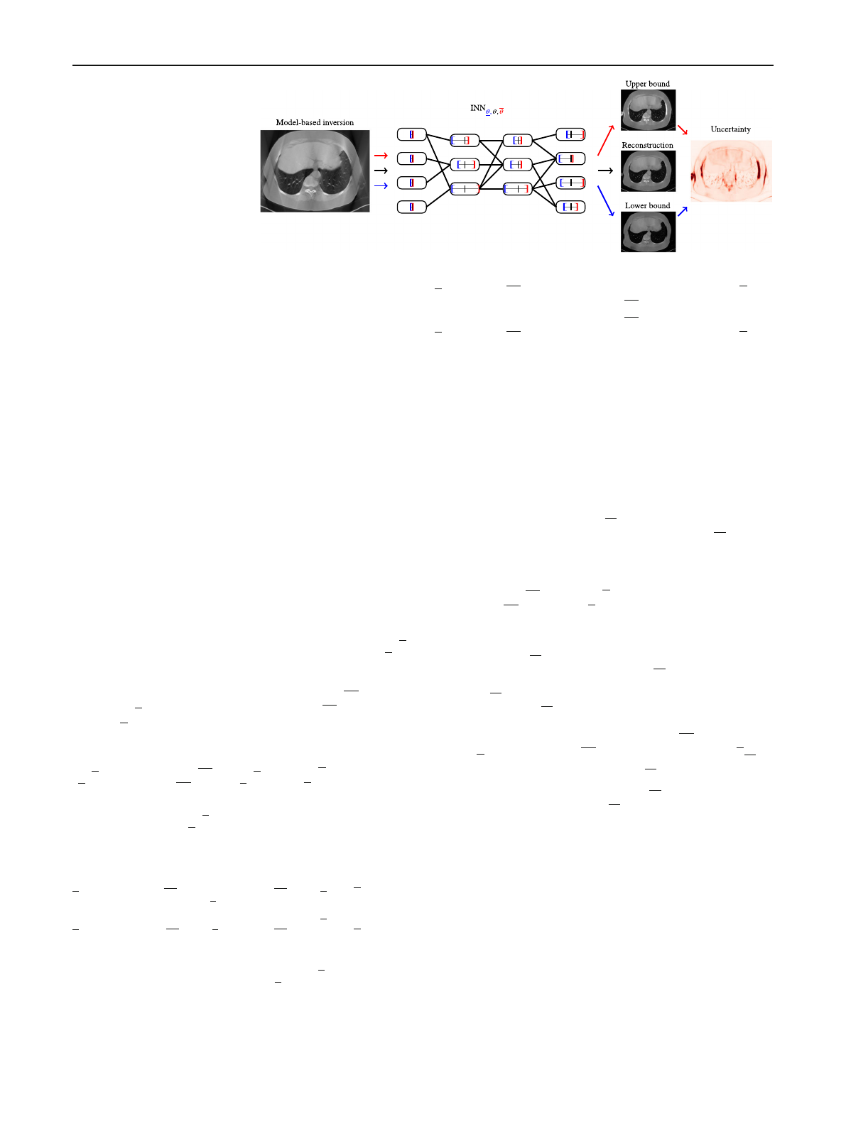
DNN Φthat has already been trained. A schematic illustra-
tion is provided in Fig. 1:TheINN is formed by wrapping
additional weight and bias intervals around the weights and
biases of the underlying prediction DNN. This allows us to
equip the DNN Φwith uncertainty capabilities without the
need to modify Φitself. After training the INN we obtain
prediction intervals that are guaranteed to contain the orig-
inal prediction of the underlying network and are easy to
interpret. They provide exact upper and lower bounds for the
range of possible values that the DNN prediction may take
when slightly modifying the network parameters within the
prescribed weight and bias intervals.
123
International Journal of Computer Assisted Radiology and Surgery (2021) 16:2089–2097 2091
Fig. 1 A schematic overview of
the proposed Interval Neural
Networks for image
reconstruction
Previously, the capacity of neural networks with interval
weights and biases was evaluated for fitting interval-valued
functions [11]. In contrast to [11], our targets xiare nei-
ther interval-valued nor univariate, leading to a different loss
function which allows us to equip trained neural networks
with uncertainty capabilities post hoc. For a direct compari-
son, see 3in 3.2 and Equation (18) in [11]. Further, [17,30]
explored neural networks implementing interval arithmetic
for robust classifications. However, in their setting, the focus
is purely on representing the inputs or outputs as intervals but
not the weights and biases. In contrast, our proposed INNs
determine interval bounds for all network parameters with
the goal of providing uncertainty scores for the predictions
of an underlying DNN.
Arithmetic of Interval Neural Networks
We will now give a description of those INN mechanisms
that deviate from standard DNNs. The forward propagation
of a single input zthrough a DNN is replaced by the forward
propagation of a component-wise interval-valued input [z,z]
through the INN. This can be expressed similarly to standard
feed-forward neural networks but using interval arithmetic
instead.Forinterval-valued weight matrices[W,W]and bias
vectors [b,b], the propagation through the -th network layer
can be expressed as
z,z(+1)=W,W() z,z() +b,b().(2)
For nonnegative [z,z](), for example when using a non-
negative activation function such as the ReLU in the
previous layer, we can explicitly rewrite (2)as
z(+1)=min W(),0z() +max W(),0z() +b(),
z(+1)=max W(),0z() +min W(),0z() +b(),
wherethemaximumandminimumarecomputedcomponent-
wise. Similarly, for point intervals z() =z() =: z(),for
example, as inputs to the first network layer, we can rewrite
(2)as
z(+1)=W() max{z(),0}+W() min{z(),0}+b(),
z(+1)=W() max{z(),0}+W() min{z(),0}+b(),
regardless of whether z() is nonnegative or not. Optimizing
the INN parameters requires obtaining the gradients of these
operations. This can be achieved using automatic differen-
tiation (backpropagation) in the same way as for standard
neural networks.
Training Interval Neural Networks
Let W() and b() be the weights and biases of the underlying
prediction network Φand let Φ:Rn→Rnand Φ:Rn→
Rndenote the functions mapping a point interval input zto
the upper and the lower interval bounds in the output layer of
the INN respectively.Givendata samples {zi,xi}m
i=1the INN
parameters[W,W]() and [b,b]() aretrained byminimizing
the empirical loss
m
i=1
max{xi−Φ(zi), 0}
2
2+
max{Φ(zi)−xi,0}
2
2
+β·
Φ(zi)−Φ(zi)
1,(3)
subject to the constraints W() ≤W() ≤W() and b() ≤
b() ≤b() for each layer. This way Φ(z)≤Φ(z)≤Φ(z)
is always guaranteed. The first two terms in (3) encour-
age that the predicted interval [Φ(zi), Φ(zi)]should contain
the target signal xi, while penalizing each component that
lies outside with the squared distance to the nearest interval
bound. The second term penalizes the interval size, so that
the predicted intervals cannot grow arbitrarily large. While a
quadraticpenalty ofthe interval size is alsopossible andleads
to similar theoretical bounds as in (4), we choose to minimize
the 1-norm to make the intervals more outlier inclusive. In
addition, the tightness parameter β>0 can further tune the
outlier-sensitivity of the intervals. This allows for a calibra-
tion ofthe INN uncertaintyscores according toan application
specific risk-budget. In practice, we found that choosing β
similar to the mean absolute error of the underlying predic-
123

2092 International Journal of Computer Assisted Radiology and Surgery (2021) 16:2089–2097
tion network yields a good trade-off between coverage [9]
and tightness.
Properties of Interval Neural Networks
The uncertainty estimate of an INN is given by the width of
the prediction interval, i.e., u(z)=Φ(z)−Φ(z).Interms
of computational overhead, INNs scale linearly in the cost
of evaluating the underlying prediction DNN with a constant
factor 2. In contrast, the popular MCDrop [10] scales lin-
early with a factor Twhich is proportional to the number
of stochastic forward passes and at least T=10 is recom-
mended by the authors, see “Baseline UQ methods” section.
Further, INNs come with theoretical coverage guarantees
that can be derived from the Markov inequality: Assuming
that the loss (3) is optimized during training to yield an INN
with vanishing expected gradient with respect to the data
distribution, we obtain
P(z,x)Φ(z)i−λβ < xi<Φ(z)i+λβ≥1−1
λ,(4)
for any λ>0. In other words, for input and target pair (z,x)
the probability of any component of the target lying inside
the predicted interval enlarged by λβ is at least 1−1
λ.Asβis
usually very small, this ensures a fast decay of the probability
of the components of xlying outside the predicted interval
bounds. Consequently, a component with a small uncertainty
scorewascorrectlyreconstructeduptosmallerrorwithahigh
probability. Of course, the training distribution needs to be
well representative of the true data distribution to extrapolate
this property to unseen data.
Finally, the optimization of the loss (3) yields additional
information: If the prediction Φ(z)lies closer to one bound-
ary of the predicted interval, the true target xhas a higher
probability of lying on the other side of the interval. Con-
sequently, INNs can provide directional uncertainty scores.
A quantitative assessment of this capability is given in
Fig. 3c+d. We note that it is also possible to explore asym-
metric uncertainty estimates in the probabilistic setting, e.g.,
via exponential family distributions [29] or quantile regres-
sion [24]. In contrast to INNs, these methods cannot be
applied post hoc as they require substantial modifications
to the underlying prediction network.
Baseline UQ methods
In addition to our INN approach, we consider two other
related and popular UQ baseline methods for comparison.
First, Monte Carlo dropout (MCDrop)[10] obtains uncer-
tainty scores as the sample variance of multiple stochastic
forward passes of the same input signal. In other words, if
Φ1,...,ΦTare realizations of independent draws of ran-
dom dropout masks for the same underlying network Φ,
the component-wise uncertainty estimate is uMCDrop(z)=
(1
T−1(T
t=1Φt(z)2−1
T(T
t=1Φt(z))2))1/2.Second,adirect
variance estimation (ProbOut) was proposed in [22] and
later expanded in [12]. Here, the number of output com-
ponents of the prediction network is doubled and trained
to approximate the mean and variance of a Gaussian dis-
tribution. The resulting network ΦProbOut :Rn→Rn×
Rn,z→ (Φmean(z), Φvar(z)) is trained by minimizing
the empirical loss i(yi−Φmean(zi))/√Φvar(zi)2
2+
log Φvar(zi)1. The component-wise uncertainty score of
ProbOut is uProbOut(z)=(Φvar(z))1/2. Note that, in con-
trast to INN and MCDrop,theProbOut approach requires
the incorporation of UQ already during training. Thus, it
cannot be employed as a post hoc evaluation of an already
trained, underlying network Φ. The role of the actual predic-
tion network is taken by Φmean.
Experiments
We present experiments for two different inverse problems.
First, a deconvolution task with 1D signals, and second a
tomographytask on real-world2Dimagesignals.Both setups
are described in more detail below. The description of all
hyperparameters for the experiments is kept brief and we
refer to our publicly available code at https://github.com/
luisoala/inn for full details.
Case study A: deconvolution of 1D signals
We start with a synthetic, didactic experiment, inspired by
a one-dimensional deconvolution task, to demonstrate the
properties of INNs discussed in “Properties of Interval Neu-
ral Networks” section. For this purpose, we choose n=m=
512 and A=DSD, where Dis a discrete cosine trans-
form (Type I DCT) and Sis a diagonal matrix with entries
sj=n−j
n−1ν
∈[0,1], that decay with a fixed exponent
ν=8. We draw synthetically generated signals xfrom a dis-
tribution of piecewise constant functions with random jump
positions and heights, see Fig. 2. The corresponding mea-
surements yare computed according to (1). We generate a
data set consisting of 2000 sample pairs (yi,xi), 1600 of
which were used for training, 200 for validation and 200 for
testing. The underlying prediction network Φis a convolu-
tional neural network (consisting of ten convolutional layers
and three dropout layers in between) trained to directly map
yto x, i.e., we use A†=Id and thus z=A†y=yin
this experiment. We trained the underlying network Φfor
100 epochs using Adam [15]. The interval parameters of the
INN were subsequently trained for another 100 epochs with
β=2·10−3.FortheMCDrop comparison, we use T=64
123
International Journal of Computer Assisted Radiology and Surgery (2021) 16:2089–2097 2093
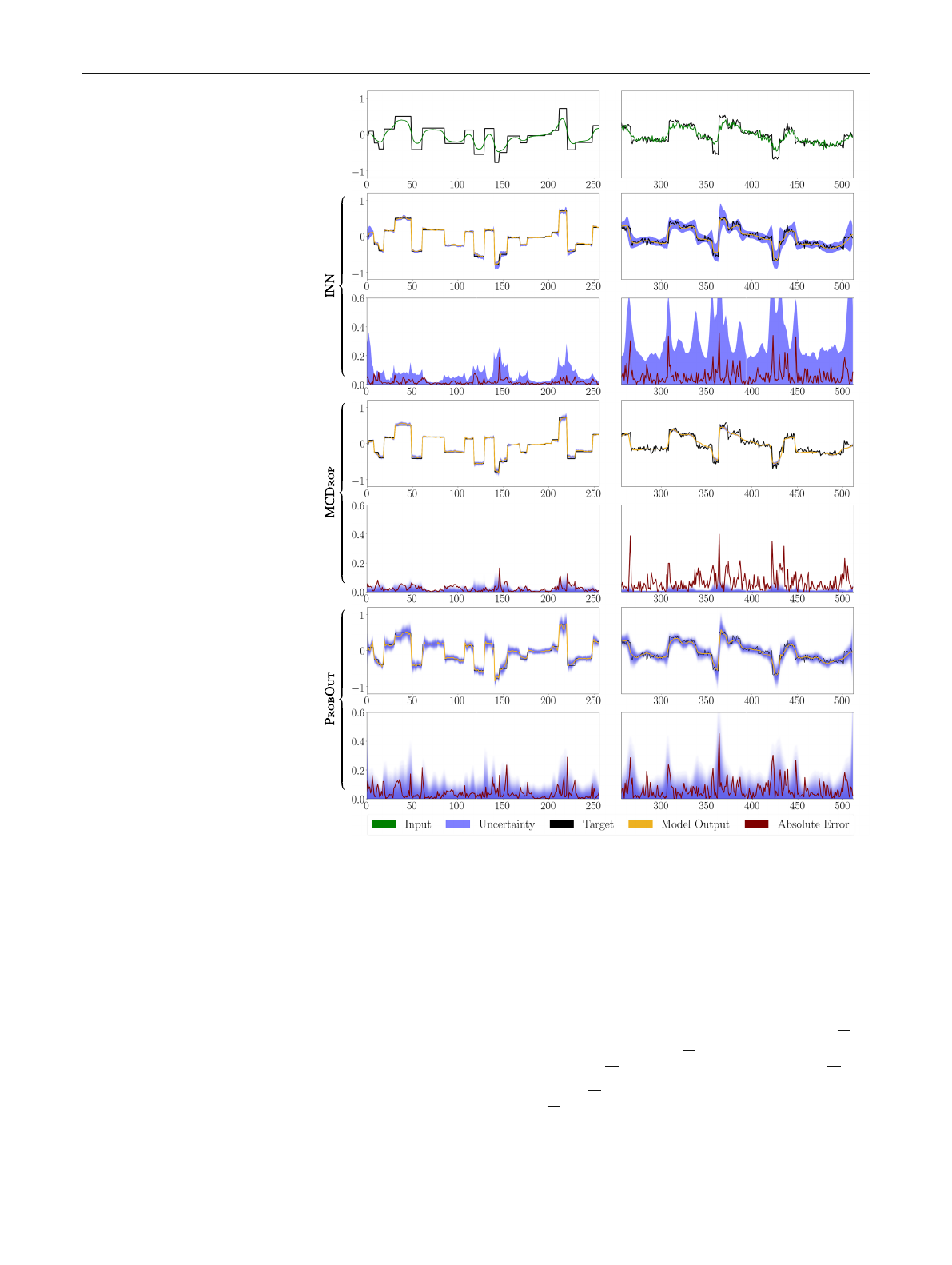
Fig. 2 Results for the
deconvolution task for one
exemplary signal without noise
(left) and with additive Gaussian
noise (σ=0.05) on both the
measurements yand signal x
(right). The first row shows
inputs z=yand targets x.
Below the target x, prediction
Φ(z)and uncertainty score u(z)
as well as the uncertainty
compared to the absolute error
|Φ(z)−x|are shown for the
three UQ methods.
samples. The ProbOut model was trained in the same way
as Φusing 100 Adam epochs. Note that all subsequent eval-
uations, as well as the plots in Fig. 2are computed using test
samples.
In order to evaluate the UQ methods’ abilities to capture
uncertainty due to noisy data, we consider additive Gaussian
noise η∼N(0,σ2·Id)on the measurements over a range of
noise levels σ(Fig. 3a) as well as η1,η2∼N(0,σ2·Id)on
the measurements and targets, where (1) is adjusted to y=
A(x+η1)+η2(Fig. 3b and right column of Fig. 2). In this
case, INNs are able to capture the additional uncertainty of η1
using the bias parameters of the final network layer. In Fig. 3,
it can be observed how in contrast to MCDrop, our method
and ProbOut are able to capture independent noise in the
data with ProbOut reacting to a lesser degree than the INN.
Note also that in Fig. 3some of the ProbOut evaluations
are shifted to the right, indicating a reduced reconstruction
performance compared to the other methods.
Finally, we determine the directional information of the
INN uncertainty scores as discussed in “Properties of Inter-
val Neural Networks” section. For this, we define the
component-wise directionality ratio by DR(z)=max{Φ(z)
−Φ(z), Φ(z)−Φ(z)}/min{Φ(z)−Φ(z), Φ(z)−Φ(z)},
i.e., as the ratio between the larger and smaller part of the
interval [Φ(z), Φ(z)]when divided by the prediction Φ(z).
The directionality accuracy (DA) is the relative frequency
123
Loading more pages...