
Technische Universität Berlin
berlin
FACHBEREICH 3
MATHEMATIK
VOLUME SEGMENTATION OF
3-DIMENSIONAL IMAGES
by
CHRISTOPHE FIORIO JENS GUSTEDT
NO. 515/1996

Volume Segmentation of 3-dimensional Images
Christophe Fiorio
TU Berlin, Sekr MA 6-1
10623 Berlin, Germany
Jens Gustedt
TU Berlin, Sekr MA 6-1
10623 Berlin, Germany
Abstract
We present a practical method to segment large medical
images that takes the whole 3-dimensional structure into
account. We use a Union-Find data structure to record
and maintain the necessary information during the seg-
mentation process. Due to the large data size, we are
forced to divide our process in two parts: a “weak seg-
mentation” of the individual sections and a global inte-
gration of all the data. This method shows good results
on computer tomographies.
1 Introduction and Overview
In this paper we present a method to perform real 3-
dimensional segmentation of tomography images (for
a more general issue on medical imaging, see e.g.
[Her83]). The data in these images is a set of cross-
sectional (slice) digital images of a part of a human
body. Certain parts of this image, such as organs, bones,
..., may need to be visualized and manipulated in order
to study the patient. But the extraction of such parts, as
well as the definition of their boundaries is fundamental
to visualization, manipulation and analysis.
In the 2-dimensional case, the problem of the def-
inition of boundaries and relative notions as connect-
edness have long been studied, see [KR89] for a sur-
vey. In the 3-dimensional case, the topology of im-
ages is still well-studied, see e.g. [Kov89, KKM90,
Lat93, AAF95]. Once the model of boundaries and
connectedness is chosen, an algorithm which realizes
the extraction of the boundaries of an object is neces-
sary. There are many works on this problem, see e.g.
[AFH81, KU92, RKW91, Udu94]. But all these algo-
rithms take a binary digital image as input such that the
“lightened” voxels are those which belong to the object
to be described., i.e. the object in question has already
The research presented in this paper was made possible by a vis-
iting grant of DIMANET per Christophe Fiorio at Berlin.
been extracted.
Several methods which perform such extraction exist,
see [UH91], but the common and non-satisfactory ap-
proach is to segment each slice separately and identify
in each of them the region(s) or the edges which match
the object (organ in our case) that is to be extracted, see
e.g. [GL93]. There is another approach described in
[MBA93] which also take a binary image but where a
3D-edge segmentation is assumed to be done (as for ex-
ample the one described in [MDMC90]) and perform a
topological reconstruction.
Our approach is slightly different, since we will take
the 3-dimensional image into account and then identify
volumes in this image as a whole. So afterwards, only
the volume that is to be displayed must be selected, no
additional operation to retrieve the 3 information is nec-
essary.
We define a volume in the classical way as a set of
connected voxels, where the connectivity relation is the
6-connectivity relation (see [KR89] for a definition).
Our method will perform volume growing, by extend-
ing the region growing in the 2D case. We are start-
ing with small volumes and we merge them together ac-
cording to a predicate. This predicate will use statistical
informations of the volume to take its decision. Note
that our method allows to use local criteria as well as
global ones. Indeed our structure provide us with a con-
nected component labeling, so for a given pair of voxels
we have local informations related to the voxels them-
selves, and global informations relative to the segment1
they belong to.
First we shortly present the basics of Union-Find and
how it can be applied to image segmentation. Then, our
approach is presented: we justify the use of a procedure
in 2-parts , “weak segmentation” and show how we deal
with with the entire 3-dimensional image. It follows a
description of an application to computer tomographies
and a presentation of results. Finally some perspectives
are given.
1which can be retrieve by a Find operation.
Page 1

2 Using Union-Find for Segmenta-
tion
The use of Union-Find data structures for image seg-
mentation is immediate: segments are just sets if we
suppress the connectivity for a moment; the Union oper-
ation then corresponds to the merging of two segments;
the Find to the identification of a particular segment. To
add the connectivity constraint, we only have to ensure
that only pairs of adjacent pixels are taken in order to
ask for the merging of two segments. Then the corre-
sponding segment are guaranted to be adjacent and the
merging of the two is indeed connected.
2.1 Basics
The general Union-Find problem, or more precisely the
disjoint set-union problem, can be formulated as fol-
lows. Given is a set S, the ground-set, of elements that
form one-element subsets at the beginning; the goal us
to perform arbitrary sequences of Union and Find opera-
tions in the best time complexity possible. Here a Union
works on two disjoint subsets fusing them into one, a
Find identifies the subset a certain element belongs to.
For an introduction and overview to Union-Find see e.g.
[Meh84, GI91]; for recent results see [vKO93].
Efficient implementations of the Union-Find problem
use tree data structures to represent sets (i.e. segments
in our case), the root of the tree being the representative
of the region. To perform an Union operation it suffices
to link the two roots of the corresponding tree, creating
thereby a new tree. The Find operation identifies the re-
gion by finding the root of the tree in an iterative pointer
search.
In the general case, the best complexity known has
been first obtained by Tarjan, see [Tar75], who has
shown that general Union-Find algorithms perform in
O
(
α
(
n
;
m
)
m
)
where αis a very slowly growing func-
tion. and n
<
mare the amounts of calls to a a Union and
Find operation respectively. In [Gus95] it is shown that
the Union-Find problem can been solve in linear time
on a RAM for special classes of graphs, in particular
for d-dimensional grids for fixed d and 8-neighborhood
graphs of a 2 dimensional grid.
So theoretically there is no problem since an im-
age can be considered as a 2-dimensional grid and
a 3-dimensional image as a 3-dimensional grid. But
the algorithms described in [Gus95] are very complex
and the application to image segmentation is not triv-
ial. But there exist linear algorithms (see [DST92,
FG96]) that perform in linear time in the special case
of 2-dimensional image segmentation. The theoreti-
cal complexity of these algorithms translate very well
in short running-time. The method described here is
based on the algorithms given in [FG96]. Let us now
present shortly how the Union-Find problem can be ap-
plied to image segmentation and more precisely to 3-
dimensional image segmentation.
2.2 Application to 3-dimensional Images
Let us first examine the 2D case. Clearly at the begin-
ning of the process of region growing all the pixels form
regions of only one element. So you have to choose
a scanning strategy (line-by-line, linear quad-tree, ran-
dom), examine all pairs of pixels of the image, and for
each pair decide whether or not to perform the merg-
ing of the two regions the pixels belong to. Note that
the scanning strategy plays an important role in the pro-
cess and its outcome. A deterministic strategy will lead
to better efficiency, but will influence the shape of the
obtained regions in particular line-by-line strategy. An
ideal strategy would be a random scan ensuring an ho-
mogeneous growing of the regions.
Note that Union-Find segmentation has the particu-
larity to be driven by the pixels. So we can use both
local (i.e. relative to the pixels) and global (i.e. relative
to the regions) merging criteria, this leads to a contour-
region cooperation. Moreover, since we can identify the
region each pixel belongs to, such a method, in paral-
lel to the segmentation process, provides us with a con-
nected component labeling.
This method can – in theory – easily be generalized
to 3-dimensional images. The same technique applies,
just replace pixel by voxel in the above text. But to im-
plement such an approach, there is a problem due to the
limitation of memory. A Union-Find data structure is a
greedily space consuming. At the beginning, each voxel
is a segment, so one may have the structure for a seg-
ment for each voxel. And in addition to the grey level
of the pixel and the pointer to the father in the tree, this
structure must record all the data needed for the merg-
ing criteria, such as e.g. number of pixels in the region,
sum of the grey levels of all the pixels of the region,
etc. For example, in our application the size of such a
structure is about 16 bytes. So it is difficult to handle
all the 3-dimensional image in memory2at once, that is
why we have used a 2-parts procedure as described in
the following.
3 Description of our Approach
As we have already mentioned, we cannot create a
Union-Find structure for the entire 3-dimensional im-
2In our application, the size of the image is 512
512
178, so all
the image structure will require about 710 MB of memory!
Page 2
age at once and load it into memory. So we will proceed
slice by slice, from the first to the last. For each slice a
weak segmentation will reduce the number of segments
to be integrated in the global Union-Find structure, and
it will then be possible to feed the entire structure ob-
tained into memory. This scanning that is actually cho-
sen is not the only possible but it is the simplest. For
a discussion of the scanning order, see section 5. The
general procedure can be summarize as follow:
Algorithm 1: Volume Segmentation
for i
=
1to number of slices do
1load slice Si;
2
weak segmentation
of Si;
3write Sito disk;
4integration of the surviving segments into the
global data structure;
if i
6
=
1then
5
volume segmentation
according to Si
1;
6free memory occupied by Si
1;
end
end
7save the result slice by slice;
The steps 1,2 and 3 form the first part of our al-
gorithm. Its goal is to reduce the amount of data in
each slice in order to be able to deal with the entire 3-
dimensional image.
The second part consist in the step 4,5 and 6. It re-
alizes the global integration of the data as a whole by
managing the global Union-Find structure and creating
volumes by the merge of the segments of the slices.
Our algorithm handles two Union-Find structures at
two different levels, a ”slice level” and a general level,
i.e. the global 3-dimensional structure. The so called
”slice structure” is a classical Union-Find structure for a
2D image as described for example in [FG96]. A record
is created for each voxel of the slice and so the slice
structure is relatively big compared to the 2D image.
After such a slice has been integrated into the global
data structure its segment information is written on disk
to free the memory that was used by it and to make the
saving slice by slice of the final result possible in the
step 7.
The global structure will keep all the segments found
after a weak-segmentation of each slice. It is dynam-
ically constructed, slice after slice. So the number of
elements of this structure will be equal to the total num-
ber of segments extracted by the weak segmentation of
all the slice. In our case it is about the same size as
an individual slice. So this structure will be not more
greedy in memory consumption as a slice structure by
itself.
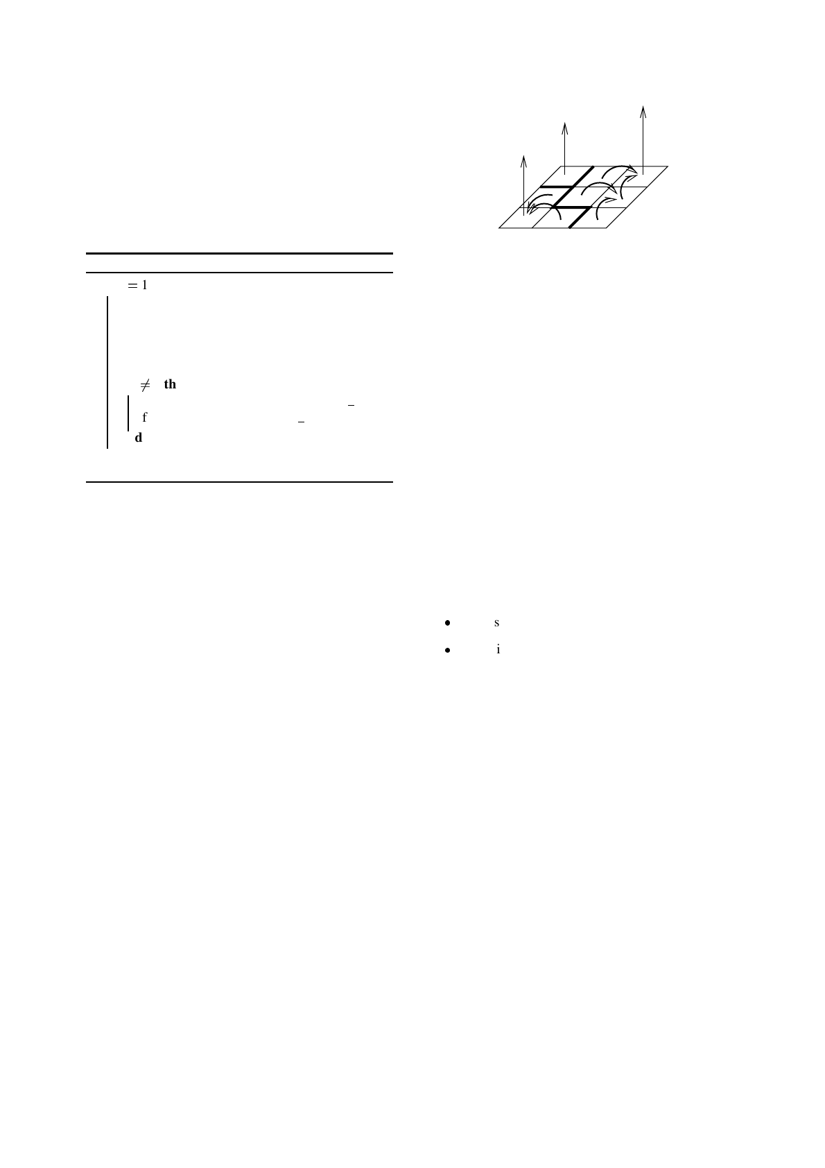
segment 3
segment 1
segment 2
Figure 1: after a weak-segmentation
3.1 Weak Segmentation of Individual
Slices
Since we need to reduce the amount of data, we are
forced to segment each slice. But we choose parameters
of the merging criteria such that the regions obtained
are still relatively small. This is what we call a “weak
segmentation”.
The intention for this is that we want to do a real
3-dimensional segmentation in order to obtain a vol-
ume description of the image. By doing a complete
segmentation of each slice, we would not take the 3-
dimensional information of the image into account. In
fact we would fall back into classical methods which
segment each slice separately and would have to per-
form a 3d-reconstruction of the image afterwards.
So we use the segmentation process in each slice as a
preprocessing tool performing a filtering on the original
image. In keeping regions small we ensure that:
no abusive merging will be performed on any slice,
the 3-dimensional information is still pertinent.
For a discussion of the merging criteria that was used in
out application and that in fact was able to guarantee the
properties we want see the discussion below.
The segmentation process used is fast and provides a
connected component labeling (see [FG96]). This last
point is important since we will need it when doing the
3-dimensional segmentation.
Now, after the weak segmentation, the number of re-
gions in a slice is substantially reduced. We have the
data structure like the one represented in Figure 1.
Before integrate these data into the global structure,
we will perform an additional process which will ensure
a better complexity in the final algorithm and thus a bet-
ter performance. This process, called ”flatten the slice”
consists in linking all the voxels directly to the segment
they belong to. This realizes the component labeling of
the slice effectively.
Note that the complexity of such a process is linear
in the number of voxel of the slice. Indeed, for each
Page 3
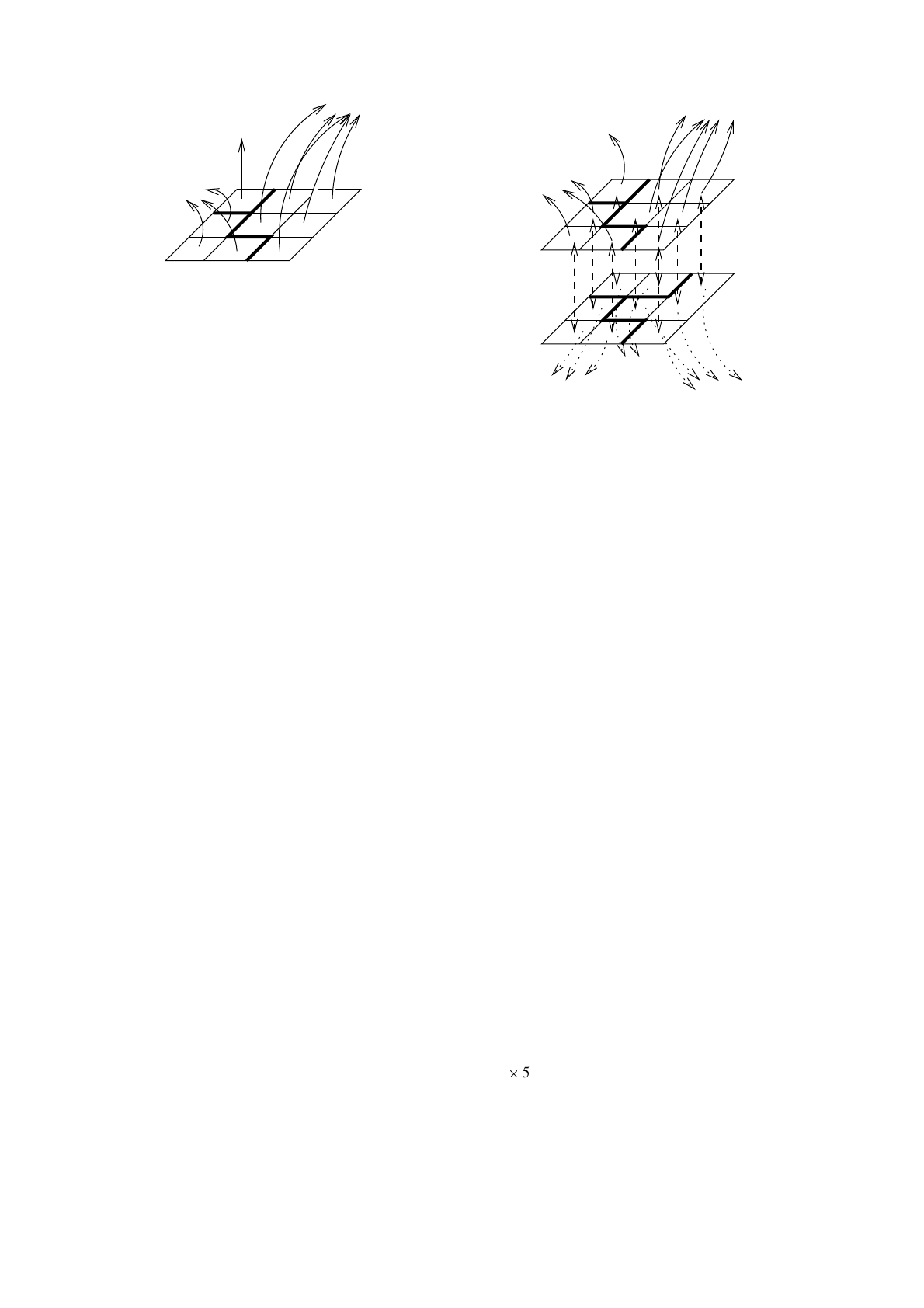
segment 1
segment 3
segment 2
Figure 2: structure obtained after a flatten
voxel we do an iterative pointer search of the root, and
on the path followed we link all the voxel directly to
the root (path compression). So each edge of the tree
which is not link to the root or a leaf, will be visited
only one time since after an iterative pointer search all
other voxels which are linked to a voxel of this path will
find directly the root from it. Each extremal edge (i.e.
edge linked to a leaf or the root) will be used one time
for each leaf. So the total number of pointer jumps is
at most equal to two times the number of edges in the
tree which is equal to the number of element of the tree
minus one, that’s give us a linear time complexity. For
a complete discussion see [FG96].
Figure 2 presents the structure obtained.
Note that the structure of a slice is still big since you
always have a structure for each voxel. But we will not
keep such a structure for each slice of the 3-dimensional
image, in fact we will have at most 2 slice at the same
time in the memory as it will be shown in the following.
3.2 Global Integration of all the Data
The surviving segments of the precedent part will be
introduced in the global data structure. They are now
considered as volumes of the image, but they are not to-
tally integrated in the segmentation since we have not
yet tried to merge them with the volume previously de-
termined to which they are adjacent. In order to realize
this, we always keep the last slice involved in the pro-
cess in addition to the new one.
Two such structures can be combined to perform a
volume segmentation. Thanks to the connected com-
ponent labeling, one just has to match corresponding
voxels to find for each segment those volumes to which
it is adjacent. For each pair of matching voxel we de-
cide whether or not merge the segment they belong to
(see Figure 3). Clearly after that we don’t need the ”old
slice” anymore and we can free it. Thus, we always
have at most 2 slice-structures in memory. In our practi-
cal application the weak segmentation of each slice give
us about the same number of segments in all the slices
slice Si-1
previous
slice Si
actual
segment 5
segment 4
segment 6
segment 2
segment 3
segment 1
Figure 3: matching of two segmented slices
as the size of one individual slice. In section 4.3 on
the next page you will give some information about the
memory demand in our application.
At the end of the algorithm we get an Union-Find
structure which describes the volume segmentation of
the image. We must now save this information. After
each weak segmentation, the slice is saved on the disk.
For each voxel of the slice we keep the segment identi-
ficator it belong to. Now, at the end of the 3-dimension
segmentation, we always have all these segments and
for each of them we know which volume it is a part of.
So we load each slice, and for each voxel replace the
segment identificator by the volume identificator.
Thus we have realized a volume segmentation of this
image and furthermore we are able to say for each voxel
which volume it belongs to.
4 Application to Computer Tomo-
graphies
In this section, we present some results obtained by our
algorithm on a computer tomography image of a part of
a human body, see Figure 6 for a look at the skeleton
found inside this part.
4.1 Description of the Data
We have 178 slices of a computer tomography start-
ing at the 8th chest vertebra and going down to the
knee. Each slice is a 256 grey levels image of size of
512
512. Figure 4 on the following page shows the
28th slice. It represents a cut through the body at about
Page 4
Loading more pages...