Advances Toward a Lightweight, Variable Fidelity Wake Simulation Tool [original]

Content from this work may be used under the terms of theCreativeCommonsAttribution 3.0 licence. Any further distribution

of this work must maintain attribution to the author(s) and the title of the work, journal citation and DOI.

Published under licence by IOP Publishing Ltd

The Science of Making Torque from Wind (TORQUE 2020)

Journal of Physics: Conference Series 1618 (2020) 052070

IOP Publishing

doi:10.1088/1742-6596/1618/5/052070

Advances Toward a Lightweight, Variable Fidelity

Wake Simulation Tool

Joseph Saverin, D Marten, N Nayeri and CO Paschereit

Chair of Fluid Dynamics, Technical University of Berlin, Berlin, Germany

E-mail: [email protected]

Abstract. A method is presented which aims to bridge the gap between overly simplified

momentum-based wake models and overly demanding finite volume models of wind turbine

wake evolution. The method has been developed to allow an essentially user-defined resolution

of the wake. Beyond this, all dominant field quantities are automatically resolved by the solver

including convection velocity, shear stress and turbulence intensity. Two distinct methods

of solution are presented which both have strengths and weaknesses, the choice of which

model being fidelity and application dependent. Both methods make use of multilevel spatial

integration to allow greatly improved computational efficiency. The method is here presented

for 2D flow in the symmetry plane of a vertical axis wind turbine as an initial demonstration of

the potential of the method.

1. Introduction and Physical modelling

The progression of the wind turbine industry towards higher order aerodynamic models in the

aerodynamic design of wind turbines is necessitated by the greater challenges facing modern

wind turbine designers including but not limited to: turbulent inflow, offshore turbines and

aeroelastics, the latter becoming increasingly prominent due to the general trend toward larger

turbine blades. Accurate modelling of unsteady loads due to the aforementioned factors make the

possibility of discarding lower order momentum-based methods in favour of higher order vortex

particle or filament methods increasingly attractive. A significant amount of research has already

been devoted to examining these models and the effects that they have on predicting fatigue

loading and performance of a wind turbine [1, 2]. For reasons of adaptability and amenability to

optimised and parallel programming, the work here adopts vorticity-based methods, which allow

a Lagrangian treatment of the flow field [3]. Furthermore, by specifying characteristic simulation

grid size, the user is essentially capable of tailoring the simulation fidelity for desired modelling

outcomes. These methods are also amenable to acceleration by their inherent formulation by

separating near and far-field influence. The general method of solution is to make use of the

fast-multipole method [4] to treat the far-field interactions. The work here however makes use

of the recently introduced multilevel integration method [5]. The application of this method to

such high order modelling has, to the author’s knowledge, not yet been significantly explored.

The application of vortex particle (VP) methods has been chosen here as it allows for all

important wake features to be inherently treated [6]. This includes unsteady aerodynamics,

trailing and bound vortex shedding, wake velocity self-induction, vorticity strength evolution,

vortex merging and destruction and modelling of turbulent effects [7]. The ability of such

The Science of Making Torque from Wind (TORQUE 2020)

Journal of Physics: Conference Series 1618 (2020) 052070

IOP Publishing

doi:10.1088/1742-6596/1618/5/052070

models to accurately predict higher order unsteady aerodynamics without incurring exorbitant

computation expense brings the treatment of inherently more difficult flow problems, such as

multiple turbine interaction, wake breakdown and wake augmentation, closer towards the design

environment and allows for improved and optimised turbine and farm design.

1.1. Equations and the Vortex Particle Method

The evolution of vorticity for an incompressible, Newtonian fluid must obey the following

equations:

∇ · ~u = 0 ,

d~ω

dt =∂~ω

∂t + (~u · ∇)~ω = (~ω · ∇)~u +ν∇2~ω (1)

These pertain to conservation of mass (continuity equation) and conservation of momentum

(vorticity transport equation), respectively. Recalling that vortex filaments behave as material

lines for an inviscid flow [8], the field can be represented as a particle set and tracked in a

Lagrangian sense. The vorticity field is then represented as the sum of a set of vortex particle

p, each with position ~xp, vorticity ~ω and characteristic volume ∆ Vp:

~ωσ(~x) = X

~ωp∆Vpζ(ρ) (2)

where ζ(ρ) = ζ((~x −~xp)/σp) is a regularisation function, introduced to remove singular

behaviour from the field. This form of solution is referred to as the vortex particle (VP)

method. The velocity field ~u(~x) is computer from the vorticity field via the stream function

ψwhich satisfies the relation ∇2~

ψ=−~ω. The Green’s function for −∇2in an unbounded

domain is given by: G(~x) = 1/(4π|~x|), which allows for convolution over the particle field:

ψ=G(~x)∗~ω(~x) where ∗is a convolution operator. For more details the reader is referred to

Winckelmans [9]. There now two methods which allow for the calculation of the velocity field

~u, both of which are based upon the solution of the Poisson equation for the stream function:

~u =∇ × ~

ψ.

Method 1: Greens Function The velocity can be extracted by convoluting equation 1.1 above:

~u =∇ × ~

ψ=X

Ku(ρ)×ωp∆V(3)

where ~

Ku(ρ) is the well-known Biot-Savart kernel for a regularized vortex particle. Analytical

expressions are known for this kernel based on the regularisation ζchosen [9]. The evaluation

of the velocity at a field points ~x hence amounts to a sum over the influence of each particle.

This shall be further detailed in the following section.

Method 2: Poisson Solver If the spatial distribution of ~

ψis known, then the velocity can

be directly extracted by calculating ∂ψi

∂xjusing finite differences. The solution to the Poisson

equation over a spatial domain Phas been the focus of significant research and highly optimised

commercial solvers are available which make use of either spectral methods [10] or multigrid

methods [11]. In order to attain the solution, boundary conditions (BC) for ψmust be specified

over the boundary of P. The most generally applicable approach to this is to specify Dirichlet

BC’s for ~

ψon the domain of interest. This has the added advantage that Pcan be specified

to compactly enclose the vortical region of interest. This is a significant advantage this method

has over finite volume (FV) solvers, as only the domain of interest is required in the calculation.

This method has been successfully applied before to general 3D VP solvers [7].

The Science of Making Torque from Wind (TORQUE 2020)

Journal of Physics: Conference Series 1618 (2020) 052070

IOP Publishing

doi:10.1088/1742-6596/1618/5/052070

Analog to the expressions for ~

Kσ,u above, there exists analytical expressions for the stream

function Kernel ~

Kσ,ψ. Fast Poisson solvers require a uniform spatial grid, and hence the

disordered particle distribution must be appropriately mapped to an underlying uniform grid

[12].

1.2. Spatial Integration- Multilevel Method

Regardless of the method of solution, the particle set must be spatially integrated in order to

determine the influence at each field point. This incurs a non-negligible computational expense

which constitutes the bulk of the task. This computational expense can be massively reduced

by making use of the multilevel method, which makes use of a hierarchical spatial coarsening

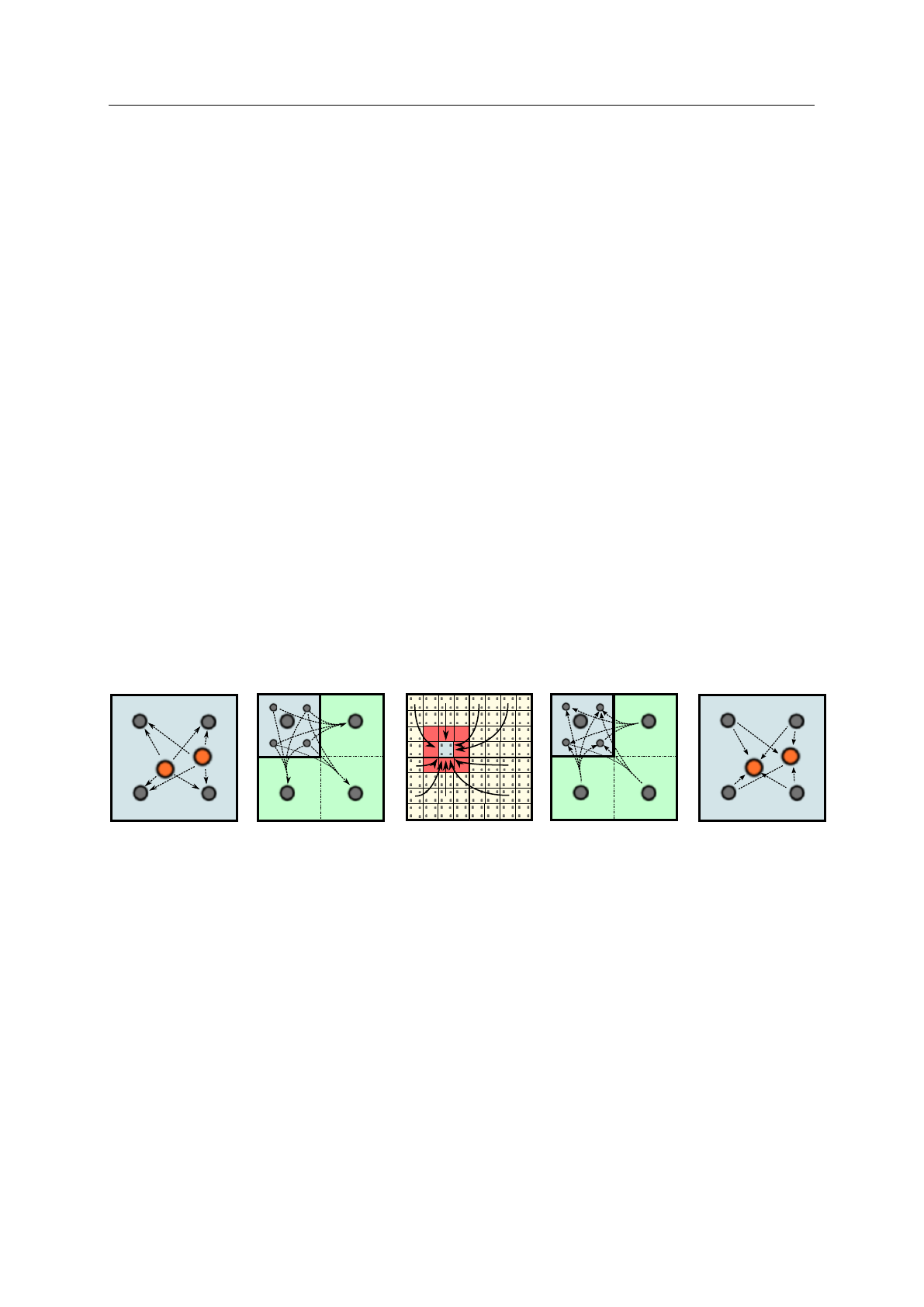
to approximate particle influence in the far-field [5]. The calculation can be broken into two

segments:

Far-Field Evaluation The particle strength distribution is adjoint interpolated (anterpolated)

onto a regular spatial grid. This is then further further anterpolated onto progressively coarser

spatial grids- as illustrated diagrammatically in Figure 1. The interaction between boxes is

calculated under the assumption that at these distances the influence can be approximated

by a singular source particle (ignoring regularization). This shall be demonstrated for the

kernels of interesting in the proceeding section. The symmetry between each box-family allows

the interaction for a given volume to be pre-calculated and expressed as a simple matrix

multiplication saving significant overhead. The accuracy of the anterpolation-interpolation is

controlled by the order of the interpolation P. This factor dictates the number of points in each

spatial direction onto which the anterpolation/interpolation occurs. For the case illustrated in

Figure 1, P= 2.

Figure 1. The method of solution of the multilevel method. From left to right: Base

anterpolation: Source particle strengths are transferred to grid nodes. Anterpolation: Grid

strengths are progressively transferred to courser grids. Interaction: Interaction between grid

boxes is carried out. Interpolation: Influence is interpolated to finer grids. Base interpolation:

Influence of far-field interpolated onto source nodes / probe nodes.

Near-Field Evaluation In the near-field, where the polynomial approximation of the source is

inaccurate the receiver-source interaction is calculated directly. The size of the region around

which the near field is directly calculated is dictated by the factor H, which represents the

minimum box size. For source particles within neighboring boxes, the interaction is calculated

directly using the Green’s functions.

The method has successfully been applied to the 3D Biot-Savart Kernel Ku,3D[13, 14, 15].

In the aforementioned works the 3D Biot-Savart Kernel was accurately captured for the

determination of the convection velocity and the application of the method to higher order

The Science of Making Torque from Wind (TORQUE 2020)

Journal of Physics: Conference Series 1618 (2020) 052070

IOP Publishing

doi:10.1088/1742-6596/1618/5/052070

effects in 3D flows is currently under way. The work here is a step towards demonstrating the

ability of the code to capture higher order effects, including viscous effects and turbulence for

2D flow, and is now described for the two modelling approaches. It shall be assumed from this

point on, that a Gaussian type smoothing is used.

Method 1: Greens Function: Multilevel far-field In this case the multilevel method is used to

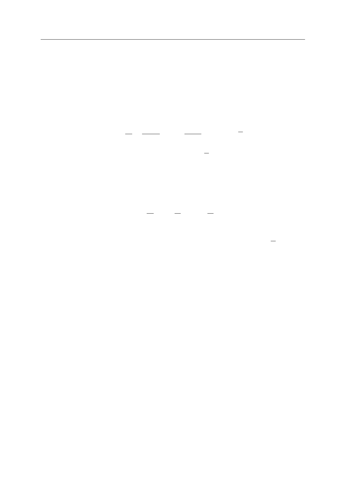
approximate the Biot-Savart Kernel in 2D for the convection velocity. This is given by:

Ku,2D=1

2πx−xp

r2~ex+y−yp

r2~ey(1 −e−ρ2

2) (4)

One immediately observes that the function g(ρ) = 1 −e−ρ2

2asymptotes very quickly to unity,

and the approximation g= 1 for ρ > 5 is generally acceptable. The solver for this method shall

hereafter be referred to as the Vortex Particle Multilevel (VP-ML) method.

Method 2: Poisson Solver: Multilevel far-field The expression for the stream function induced

by a 2D vortex particle is given by:

ψu,2D=1

4π(log ρ2

2!+E1 ρ2

2!) (5)

where E1is the exponential integral. The exponential integral decays very quickly and for

ρ > 5 its contribution can be taken as negligible. The remaining term log(ρ2

2) presents

difficulties in the far-field due to the scaling with respect to the characteristic coresize σ. By

expanding out the expression, one has for the stream function in the far-field the following:

ψff =log(r2)−log(σ2)−log(2). This can be pre-calculated for a box-receiver template as

outlined earlier, however must be scaled appropriately for each higher grid level. The leading

far-field term for grid level nbecomes: log(2nr2) = nlog(2) + 2 log(r). The practicality of the

multilevel method can hence be fully exploited. The solver for this method shall hereafter be

referred to as the Vortex Particle- Mesh Multilevel (VPM-ML) method.

1.3. Field Quantities

The resolution of the necessary quantities shall be described.

1.4. Viscous Effects

The resolution of the Laplacian of vorticity ∇2~ω is necessary to ensure viscous effects in the flow

are captured. These are crucial for the modelling of vortex merging or destruction, important

physical processes in wake breakdown.

VP-ML Method The method of particle strength exchange (PSE) approximates the Laplacian

with an integral operator. The method has been shown to accurately capture viscous effects

provided that particle overlap is maintained [16, 9].

VPM-ML Method The Laplacian is approximated on the grid by making use of an isotropic

finite difference stencil as described in Cocle [7].

The Science of Making Torque from Wind (TORQUE 2020)

Journal of Physics: Conference Series 1618 (2020) 052070

IOP Publishing

doi:10.1088/1742-6596/1618/5/052070

Turbulent shear stress In the approach taken here, a large eddy simulation (LES) approach

is taken. Here the most energetic scales are resolved and the effect of sub-grid scales (SGS) is

modelled. For the purpose of it’s simple implementation, a simple hyper viscosity model is used.

dωT

dt =−C

(h2∇2)2ω(6)

where Cis a coefficient and T0a global time scale. This makes use of the Laplacian scheme

as implemented above to calculate an additional rate of change of vorticity term. Although

not displayed here, the model also automatically captures the shear stress terms of the strain

rate tensor Sij, which implies that the model could also be used for higher order turbulence

modelling, such as that detailed in Jeanmart et al. [17] or Cocle et al. [7].

2. Validation

The validation of the solver shall proceed as follows. First validation that the multilevel method

functions for the calculation of the i) Biot-Savart kernel for the VP-ML method, and ii) the

stream function kernel for the VPM-ML method is demonstrated. Following this the capturing of

important physical quantities is described including convection, viscous velocities and turbulence

parameters.

2.1. Multilevel far-field behaviour

For both bases the relative EL2type error is given, where EL2=L2(∆~x)/L2(~x) error is shown,

where L2(~a) = 1

nPn(|~a|)2. The influence is carried out on a particle set corresponding to the

wake behind a vertical axis wind turbine (VAWT), as demonstrated in the application section.

The value of the calculated influence at each vortex particle position ~

I(~xp) is compared to the

value calculated directly from the Green’s function method ~

ID(~xp), from this the error metric

is calculated L2(~

I(~xp)−~

ID(~xp)).

Multilevel Treatment of Biot-Savart Kernel This kernel is applied when using the VP-ML

method. As seen in Figure 2, the behaviour of the multilevel method is well predicted and

generally it can be seen that the error due to the multilevel far-field approximation is seen to

generally decrease with increasing minimum box-size H, this is intuitive as the larger H, the

larger region is directly calculated. It can also be observed that the error plateaus beyond a

certain polynomial approximation order P, this is the point at which the error incurred by the

far-field approximation cannot be recovered. The choice of Hand Pis then hence a matter of

desired accuracy. It can also be observed that, provided Hhas been adequately chosen, Pscales

logarithmically, and therefore each increase in Preduces the error by a factor of 10.

Multilevel Treatment of Stream Function Kernel This kernel is applied when using the VPM-

ML method. Figure 2 shows the error as a function of polynomial order. Similar behaviour is

observed for the stream function kernel as was seen for the Biot-Savart kernel. An initially linear

behaviour, followed by a plateu. This is fundamentally of interest, as the logarithmic function

in the stream function kernel is monotone increasing, as opposed to monotone decreasing for

the 1/r2factor in the Biot-Savart kernel. This implies that the total contribution to the stream

function from far-field points may contribute more to the total influence. The behavior of the

velocity field however is in fact dependent on the gradients of the stream function ∇ψz. The

stream function in the 3D case has again a far-field behaviour similar to the Biot-Savart kernel.

Loading more pages...