
Copyright applies. A non-exclusive, non-transferable and limited
right to use is granted. This document is intended solely for
personal, non-commercial use.
Terms of Use
©IWA Publishing 2016. The definitive peer-reviewed and edited version of this article is published in
Water Science and Technology 73, 10, pp. 2430–2435, 2016, 10.2166/wst.2016.092 and is available at
www.iwapublishing.com.
Matta, E., Selge, F., Gunkel, G., Rossiter, K., Jourieh, A., & Hinkelmann, R. (2016). Simulations of
nutrient emissions from a net cage aquaculture system in a Brazilian bay. Water Science and Technology,
73(10), 2430–2435. https://doi.org/10.2166/wst.2016.092
Matta, E., Selge, F., Gunkel, G., Rossiter, K., Jourieh, A., & Hinkelmann,
R.
Simulations of nutrient emissions from a
net cage aquaculture system in a Brazilian
bay
Journal article | Accepted manuscript (Postprint)
This version is available at https://doi.org/10.14279/depositonce-7288

Simulations of nutrient emissions from a net cage aquaculture system in a
Brazilian bay
E. Matta*, F. Selge**, G. Gunkel**, K. Rossiter***, A. Jourieh* & Reinhard Hinkelmann*
* Technische Universität Berlin, Chair of Water Resources Management and Modeling of Hydrosystems, Gustav-Meyer-Allee
25, 13355 Berlin, Germany: elena.matta@wahyd.tu-berlin.de, reinhard.hinkelmann@wahyd.tu-berlin.de,
ayman.jourieh@wahyd.tu-berlin.de
** Technische Universität Berlin, Chair of Water Quality Control, Straße des 17. Juni 135, 10623 Berlin, Germany:
florian.selge@tu-berlin.de, guenter.gunkel@tu-berlin.de
*** Universidade Federal do Pernambuco, Av. Professor Morais Rego, Recife - PE, 50670-901, Brazil:
karina_rossiter@yahoo.com.br
Abstract: Hydrodynamics and transport simulations were conducted with the modeling software TELEMAC-2D on
Icó-Mandantes bay, a branch of the Itaparica reservoir. The bay has a maximal operational water level amplitude of 5
m and is suffering for eutrophication and algae bloom. Therefore, we investigated low and high water level scenarios
with two different high resolution meshes, with the purpose to deeper understand their impact on transport of
substances and to improve the watershed management. In particular, nutrient emissions from a hypothetical net cage
aquaculture system located in the bay were investigated on half-year cycles. We observed a relevant impact on water
quality for a tilapia production of 130 t y-1, i.e. after 6 months simulation we obtained around 8 µgP L-1 and 6 µgP L-1
at the source of emissions, for low and high water scenario, respectively.
Keywords: Itaparica reservoir; water level change; transport; São Francisco River
Introduction
Many reservoirs in Brazil were built within the last 50 years, primarily for water storage and energy
production, without a conscious consideration of the environment. As a general consequence,
large-dam construction in the 1960s and 1970s strongly interfered with river functioning and the
hydrological cycles, producing many changes in these cycles and in the biodiversity related to the
rivers (Tundisi & Matsumura-Tundisi 2003). Human intervention affects irreversibly water flows
natural state, with a huge social and ecological impact. In Itaparica reservoir, located in the semi-
arid Pernambuco, Northeast Brazil, climate and land-use changes as well as multiple uses of water
lead to water quality problems (Gunkel & Sobral 2013). Surface water conservation, both for water
quality and quantity aspects, is strategic for the sustainable development of the region (Araújo et
al. 2003). Therefore, it is necessary to face the social, political and ecological issues with the help
of multi- and trans-disciplinary studies, in order to find enhanced management options for the
future. This is one of the purposes of the INNOVATE project (Interplay among multiple uses of
water reservoirs via innovative coupling of substance cycles in aquatic and terrestrial ecosystems),
a joint research in collaboration between Germany and Brazil, which this work belongs to.
Object of the study is Icó-Mandantes bay, a shallow eutrophic bay, located approximately in the
middle of Itaparica reservoir. A map of the study site can be found in Matta et al. (2014). Previous
research in the area showed that exchange with the reservoir main stream hardly occurs, as long as
wind is neglected (Özgen et al. 2013; Broecker et al. 2014; Matta et al. 2014). Water multiple uses
(e.g. irrigation agriculture), water level fluctuations and shore’s desiccation, caused by high
evaporation rates (ca. 2,000 mm y-1), are overstressing the bay, isolating it from the river (Selge et
al. 2015). In this work, we simulated hydrodynamics and transport using TELEMAC-2D, in order
to quantify the mechanisms and timescales of exchange between Icó-Mandantes bay and the
1

reservoir main stream, according to different water elevations. We investigated in particular
nitrogen and phosphorus dissolved ions emissions from an aquaculture system hypothetically
located in the bay, to quantify the potential impacts on water quality.
Material and Methods
Modeling tools
The bathymetry of the model was set up using measured data mapping, conducted by echo sounder
profiling during different field campaigns, performed between 2012 and 2014 (Selge et al. 2015).
The data were imported and elaborated with the help of Janet (Smile Consult GmbH), an efficient
tool to generate and edit grids for numerical simulations. TELEMAC-2D, a module of the
TELEMAC-MASCARET system (Laboratoire National d'Hydraulique et Environnement (LNHE),
part of the R&D group of Électricité de France), was used as processor. It is a powerful integrated
modeling tool for free-surface flows and it solves the two-dimensional shallow water and transport
equations with complex algorithms mainly based on the Finite Element Method, computing the
water depth, the two velocity components and the depth averaged concentration at each point of
the mesh (Hervouet 2007). After each computation, the results were examined with the help of
ParaView, an open-source multi-platform data analysis and visualization application (Ayachit
2015).
Governing equations
The governing equations are the two-dimensional depth-averaged shallow water and transport
equations. The shallow water equations consist of the continuity and the momentum equations in
x- and y-direction (Equation 1, 2, 3):
𝜕𝜕ℎ
𝜕𝜕𝜕𝜕 +𝜕𝜕𝜕𝜕ℎ
𝜕𝜕𝜕𝜕 +𝜕𝜕𝜕𝜕ℎ
𝜕𝜕𝜕𝜕 = 0 (1)
𝜕𝜕𝜕𝜕ℎ
𝜕𝜕𝜕𝜕 +𝜕𝜕𝜕𝜕2ℎ
𝜕𝜕𝜕𝜕 +𝜕𝜕𝜕𝜕𝜕𝜕ℎ
𝜕𝜕𝜕𝜕 −𝜕𝜕
𝜕𝜕𝜕𝜕 �𝜈𝜈𝜕𝜕𝜕𝜕𝜕𝜕
𝜕𝜕𝜕𝜕 ℎ�− 𝜕𝜕
𝜕𝜕𝜕𝜕 �𝜈𝜈𝜕𝜕𝜕𝜕𝜕𝜕
𝜕𝜕𝜕𝜕 ℎ� =ℎ(𝑓𝑓𝑥𝑥
𝜌𝜌−𝑔𝑔𝜕𝜕(ℎ+𝑧𝑧𝑏𝑏)
𝜕𝜕𝜕𝜕 ) (2)
𝜕𝜕𝜕𝜕ℎ
𝜕𝜕𝜕𝜕 +𝜕𝜕𝜕𝜕𝜕𝜕ℎ
𝜕𝜕𝜕𝜕 +𝜕𝜕𝜕𝜕2ℎ
𝜕𝜕𝜕𝜕 −𝜕𝜕
𝜕𝜕𝜕𝜕 �𝜈𝜈𝜕𝜕𝜕𝜕𝜕𝜕
𝜕𝜕𝜕𝜕 ℎ�− 𝜕𝜕
𝜕𝜕𝜕𝜕 �𝜈𝜈𝜕𝜕𝜕𝜕𝜕𝜕
𝜕𝜕𝜕𝜕 ℎ� =ℎ(𝑓𝑓𝑦𝑦
𝜌𝜌−𝑔𝑔𝜕𝜕(ℎ+𝑧𝑧𝑏𝑏)
𝜕𝜕𝜕𝜕 ) (3)
where u and v are the x- and y-component of the velocity vector, respectively, 𝜈𝜈𝜕𝜕 is the turbulent
viscosity (assumed constant and equal to 𝜈𝜈𝜕𝜕 =10-4 m2 s-1), 𝑓𝑓𝜕𝜕 and 𝑓𝑓𝜕𝜕 are the shear stresses (at the
bottom and at the surface) in x- and y-direction, respectively, ℎ is the water depth, 𝑔𝑔 is the gravity
acceleration, 𝜌𝜌 is the fluid density and 𝑧𝑧𝑏𝑏 is the bottom elevation.
The bottom and the surface friction (i.e. wind) are respectively determined through the Strickler
law and the empirical Flather’s approach, where the relevant parameters are the Strickler
coefficient for the first, the wind velocity and a wind shear stress coefficient, dependent on wind
velocity and direction, for the second. More information about the consideration of wind forcing
in the TELEMAC system may be found in (Hervouet 2007). A mean wind of 5.5 m s-1 blowing
from South-East with an angle of 140° (Matta et al. 2014) and a Strickler bottom friction coefficient
of 30 m0.33 s-1 (Cirilo 1991) were chosen for each case studied.
The depth-averaged transport equation is shown in Equation 4:
𝜕𝜕𝜕𝜕
𝜕𝜕𝜕𝜕 +𝑢𝑢𝜕𝜕𝜕𝜕
𝜕𝜕𝜕𝜕 +𝑣𝑣𝜕𝜕𝜕𝜕
𝜕𝜕𝜕𝜕 −𝜕𝜕
𝜕𝜕𝜕𝜕 �𝜈𝜈𝜕𝜕,𝜕𝜕𝜕𝜕𝜕𝜕
𝜕𝜕𝜕𝜕�− 𝜕𝜕
𝜕𝜕𝜕𝜕 �𝜈𝜈𝜕𝜕,𝜕𝜕𝜕𝜕𝜕𝜕
𝜕𝜕𝜕𝜕�= 0 (4)
2
where 𝑐𝑐 is the concentration and 𝜈𝜈𝜕𝜕,𝜕𝜕 is the turbulent diffusivity (assumption: 𝜈𝜈𝜕𝜕,𝜕𝜕 =10-4 m2 s-1).
We considered only conservative transport in our study, simulating phosphorus and nitrogen
emissions. This means that biological or chemical reactions and feedback effects of the transport
with the flow are not taken into account. The evolution in time of the transported substances
depends on advection (most relevant) and diffusion, whose terms are shown in Equation 4.
Further, two-dimensional simulations are carried out, i.e. vertical variations of the velocity or
concentration are also not considered.
Preprocessing
Water level fluctuations are common phenomena in semi-arid areas due to rain seasons, high
evaporation rates and hydropower generation. These changes play an important role for water
quality by aquatic biodiversity development, nutrient release from desiccated areas and therewith
water quantity management becomes a major tool for aquatic ecosystem control in these regions.
Therefore, the study cases were investigated according to high and low water levels, in order to
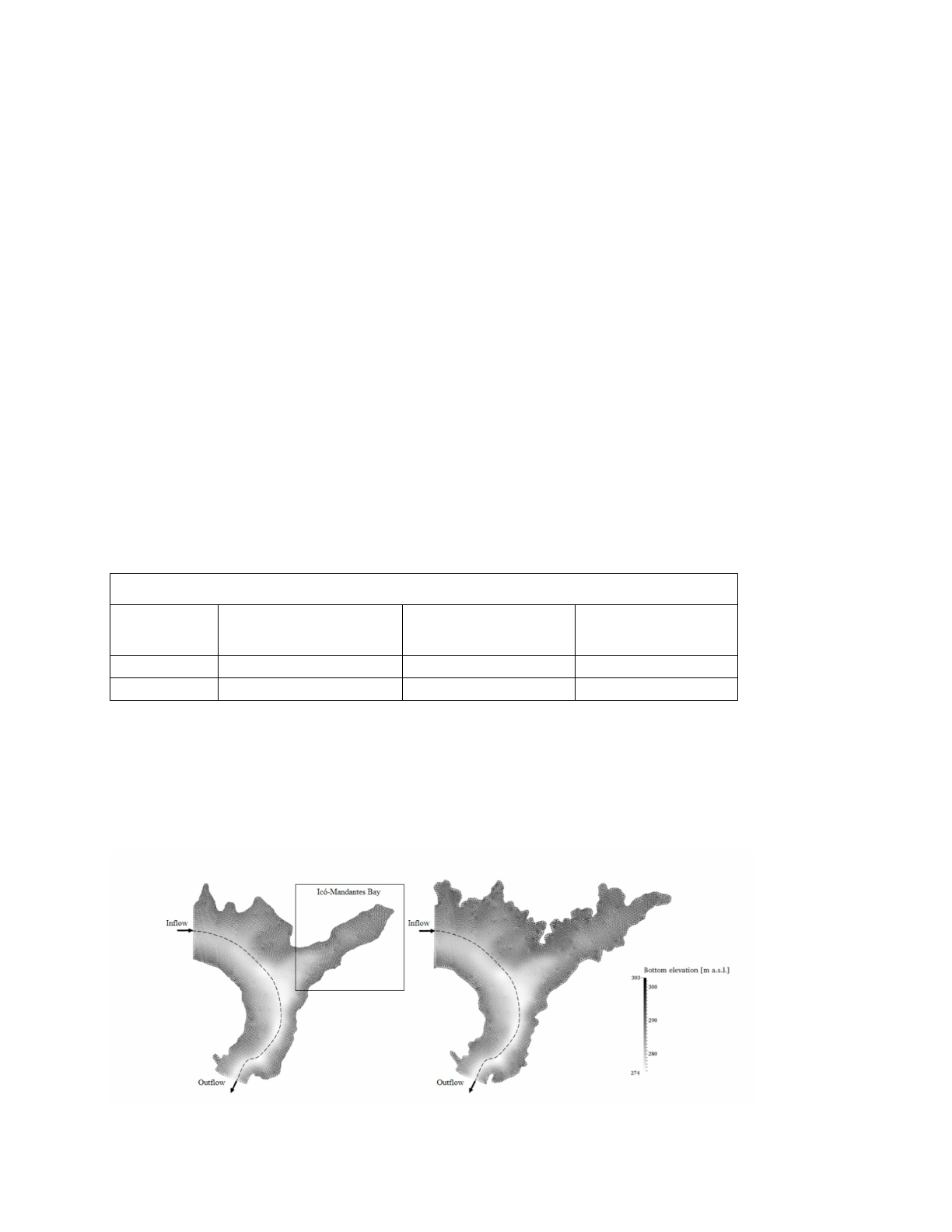
compare the respective results. Two unstructured triangular grids with high resolution were set up
with the software Janet, one for low water level (LWL) and one for high water level scenarios
(HWL) (Tab. 1).
Table 1 Characteristic parameters of the grids
High resolution models with unstructured mesh
Water level Maximum bottom
elevation (m a.s.l.)
Prescribed water
elevation (m a.s.l.)
Number of
triangular cells (-)
LWL
299.5
300.0
17,000
HWL
302.8
304.0
23,000
The computational domain has an area of around 100 km2: it covers Icó-Mandantes bay and it
includes a part of São Francisco River, concerning the inflow and the outflow (Fig. 1). São
Francisco river, the longest in Brazil with about 2,914 km length, crosses the area and it is
interrupted in its flow by the Luiz Gonzaga dam, forming the Itaparica reservoir: a large basin of
about 828 km2, with a regulated mean flow of 2,060 m3s-1 and a mean water elevation of 302.8 m
a.s.l.
Figure 1 Unstructured high resolution grid for LWL (left) and for HWL (right). The black frame in the LWL grid (left)
highlights Icó-Mandantes bay.
3

Results and Discussion
A low water level of 300 m a.s.l. and a high water level of 304 m a.s.l. were imposed as constant
water elevation for low water level (LWL) and for high water level (HWL) at the outflow boundary,
respectively, and a controlled discharge of 2,060 m3 s-1 as boundary condition at the inflow from
Itaparica.
Aquaculture nutrient emissions
Tilapia production in Itaparica reservoir amounts to 20,000 tons per year. In Brazil, 1% of the lake
surface is allowed to host aquaculture (43,267 t y-1), but there are concerns about the sustainability
to this regulation (Gunkel et al. 2013). Net cage fish culture brings a desirable economic
development, but can also contaminate water bodies with eutrophication and sediments leading to
anoxic conditions (Gunkel et al. 2015). Thus far, Icó-Mandantes bay is not yet interested by any
aquaculture system, although it is used e.g. for fishery, irrigation agriculture. Therefore, we thought
to model the accumulation of nitrogen and phosphorus dissolved ions emissions from a hypotetical
location inside the bay. Their spreading, as well as their retained mass quantities, were observed in
time and space.
The choice of the emissions site required a specific care. Since it is necessary to guarantee enough
space to allow translocation and dilution of particulate organic material to avoid an extreme
sediment increase beneath the cages (Resolução CONAMA 413, 2009; Gunkel et al. 2015), we
adopted a point of 5 m and 9 m water depth for LWL and HWL respectively, near the southeastern
shore of the bay. We assumed a productivity of 130 t y-1, which means that Dissolved Nitrogen
(DN) and Dissolved Phosphorus (DP) are equal to around 17.359 kg d-1 and 1.302 kg d-1,
respectively. The emissions were simulated as a daily accumulation of nutrients, implementing a
tracer source in TELEMAC-2D. The results were observed after 1 week and 6 months computation.
In Table 2 we reported the values of DN and DP in 4 observation points chosen inside the domain
(Fig. 2), considering the modeled aquaculture impact for LWL and HWL.
Table 2 DN and DP concentrations [µgL-1] at 4 observation points chosen inside Icó-Mandantes bay after 1 week and
6 months simulation.
LWL 1 week
HWL 1 week
Observation points
DN [µgL-1]
DP [µgL-1]
Observation points
DN [µgL-1]
DP [µgL-1]
1224
0
0
1224
0
0
3972 – source point 103.120 7.735 3972 – source point 53.164 3.988
6479 0 0 6479 0 0
8536 0 0 8536 0 0
LWL 6 months
HWL 6 months
Observation points
DN [µgL-1]
DP [µgL-1]
Observation points
DN [µgL-1]
DP [µgL-1]
1224
0.683
0.051
1224
0.403
0.030
3972 – source point 110.575 8.294 3972 – source point 74.815 5.612
6479 0.012 0.001 6479 0.008 0.001
8536 7.497 0.562 8536 4.580 0.344
4
Loading more pages...