
fluids
Article
An Accurate Finite Element Method for the
Numerical Solution of Isothermal and
Incompressible Flow of Viscous Fluid
Bilen Emek Abali
Received: 24 October 2018; Accepted: 3 January 2019; Published: 8 January 2019
Abstract:
Despite its numerical challenges, finite element method is used to compute viscous
fluid flow. A consensus on the cause of numerical problems has been reached; however, general
algorithms—allowing a robust and accurate simulation for any process—are still missing. Either a
very high computational cost is necessary for a direct numerical solution (DNS) or some limiting
procedure is used by adding artificial dissipation to the system. These stabilization methods are
useful; however, they are often applied relative to the element size such that a local monotonous
convergence is challenging to acquire. We need a computational strategy for solving viscous fluid
flow using solely the balance equations. In this work, we present a general procedure solving fluid
mechanics problems without use of any stabilization or splitting schemes. Hence, its generalization to
multiphysics applications is straightforward. We discuss emerging numerical problems and present
the methodology rigorously. Implementation is achieved by using open-source packages and the
accuracy as well as the robustness is demonstrated by comparing results to the closed-form solutions
and also by solving well-known benchmarking problems.
Keywords: finite element method; fluid dynamics; computation; viscous fluid flow
1. Introduction
Isothermal flow of viscous fluid is modeled in Cartesian coordinates by using the balance
equations of mass and linear momentum:
∂ρ
∂t+∂viρ
∂xi
=0 , (1a)
∂ρvj
∂t+∂
∂xiviρvj−σij=ρgj, (1b)
respectively, where
ρ
denotes the mass density,
vi
the velocity,
σij
the non-convective flux term
(Cauchy’s stress),
gi
the specific supply (gravitational forces); here and henceforth we apply Einstein’s
summation convention to repeated indices. In the case of Newtonian fluids such as water, oil, or alcohol,
a linear relation for stress furnishes the governing equations with sufficient accuracy. This linear
relation is sometimes called the Navier–Stokes equation:
σij = (−p+λdkk)δij +2µdij ,dij =1
2∂vi
∂xj
+∂vj
∂xi,(2)
with the material constants
λ
,
µ
; and a new parameter called (hydrostatic) pressure,
p
. In the
literature, often the law of motion, i.e., the material equation inserted into the balance equation
is called Navier–Stokes equation. Navier did use Lagrangean method for derivation of the law of
Fluids 2019,4, 5; doi:10.3390/fluids4010005 www.mdpi.com/journal/fluids

Fluids 2019,4, 5 2 of 20
motion; however, Stokes used—as we do it herein as well—the method introduced by Cauchy for
separating material equation from the balance equation, see [
1
] for historical remarks. Consider an
incompressible flow in a control volume initially filled with homogeneous water. Thus, the mass
density remains constant in space and time; from the mass balance in Equation (1a), we obtain
∂vi
∂xi
=0 , (3)
which is used for computing the pressure
p
. For an incompressible flow—as seen from Equations
(2)
and
(3)
—the mechanical pressure
−1
3σii
becomes identical to the hydrostatic pressure
p
such that we
handle
p
as the pressure generated in a pump. Velocity and pressure fields have to satisfy Equations
(1b)
and (3).
In analytical mechanics, the aforementioned equations are fulfilled locally (in every infinitesimal
volume element or simply point in space). For a computation we discretize the space, herein by using
the finite element method (FEM). Within each element, the analytical functions for the unknowns
vi
and
p
are represented by form (shape) functions with a local support, i.e., by means of a discrete
element. The shape functions are not smooth, they belong to
Cn
with a finite
n
. In other words,
the unknowns are finitely differentiable and depending on the governing equations and constitutive
relations—from the mathematical analysis in [
2
]—we know that the correct choice of the form functions
for velocity and pressure is of paramount importance for a robust computation. This so-called
Ladyzhenskaya–Babuska–Brezzi (inf-sup compatibility) condition (LBB condition) tells us how to
adjust the shape functions of velocity and pressure in the case of an isothermal and incompressible
flow. Special elements like the Taylor–Hood element [
3
] or a mixed element with bubble functions [
4
]
are often used for the isothermal and incompressible fluid flow problems. If one wants to include
temperature deviation and electromagnetism into the computation, we fail to know the corresponding
LBB condition for all shape functions (velocity, pressure, temperature, and electromagnetic fields).
For practical purposes, a robust computation without exploiting the LBB condition is useful for a
straightforward extension to multiphysics applications. This aspect is the main motivation of this work.
1.1. Computational Fluid Dynamics (CFD)
There are several methods for solving the aforementioned equations numerically. The finite
element method is very well suited for problems in solid mechanics such that a robust finite
element method in fluid dynamics allows us to implement a fluid structure interaction quite easily.
Moreover, the finite element method also delivers results in thermodynamics and electromagnetism
by using standard form functions as demonstrated in [
5
] such that a generalization to multiphysics
problem attracts attention. Therefore, we concentrate on the finite element method for fluid flow
problems. Within a finite element, the governing equations are satisfied globally (over the domain
of the element). There exists a general assumption that we can use the same local governing
equations holding globally in finite elements; however, this strategy leads to several numerical
problems and to various proposals in [
6
–
14
], for a review of such suggestions see [
15
]. These so-called
stabilization methods introduce a numerical parameter depending on the underlying mesh. There are
several successful implementations as in [
16
–
23
]. From a practical point of view, such a stabilization
method is very useful; however, introducing numerical parameters may be challenging as they
need to be tuned depending on the application, see [
24
] for a discussion about this issue leading
to methods being conditionally stable; see references in [
25
] about accuracy problems of different
techniques. Indeed, numerical strategies exist for performing accurate simulations without numerical
parameters. By using small elements—smaller than the characteristic length scale, for example
Kolmogorov scale—we can overcome the numerical problems. This direct numerical simulation
(DNS) is accurate and robust as demonstrated in [
26
–
32
]; however, it is often not feasible without
access to super-computers. There is another class of so-called splitting or projection methods such as
Chorin’s method or its derivatives as in [
33
–
39
]. The finite volume method (FVM) is often used in the

Fluids 2019,4, 5 3 of 20
computational fluid dynamics (CFD) as it is accurate and stable [
40
–
43
]. These methods are reliable;
but it is challenging to adopt a splitting method or FVM in multiphysics. By using the FEM for viscous
fluid flow, we intend to design a computation strategy by employing only physical (measurable)
parameters in such a way that the strategy shows a local monotonous convergence as expected from
the FEM.
The briefly mentioned problems are well known in the literature such that various new
computation methods are suggested for viscous flow problems. The (numerical) parameter free
approach in [
44
] shows 2D and 3D results for stationary viscous flows without the nonlinear
convection term (often called Stokes’s problem). Based on this idea an under-integrated mass matrix
is used in [
45
,
46
] to perform simulations without stabilization terms in 2D. Several mesh-dependent
stabilization terms and their connections to mesh-independent stabilization methods are investigated
in [
47
]. In [
48
] vorticity is used instead of velocity such that a new kind of splitting scheme is
proposed for solving 3D problems. In [
49
] balance equations of mass, momentum, angular momentum,
and energy are used for performing 3D computations without numerical parameters; however,
the method already uses the energy equation such that generalization for the non-isothermal case seems
to be quite difficult. In [
50
] vorticity is introduced as an independent term ensuring that the balance of
moment of momentum is satisfied, in 2D numerical solutions are performed without necessitating
any (numerical) parameters. In [
51
] different strategies are performed for establishing 3D simulations.
They are all based on writing the nonlinear convection term in a different (mathematically equivalent)
form. In [
52
] a gradient-velocity-pressure formulation is suggested to solve 2D numerical experiments.
1.2. Scope of This Work
In this work, we discuss a special yet general case, namely an isothermal and incompressible
flow. For understanding the numerical problems, often, the pressure related numerical problems and
velocity related numerical problems are studied separately. We use one balance equation for calculating
the pressure and another balance equation for calculating the velocity. It is important to remark that
both balance equations are coupled such that it is not uniquely defined which one to use for computing
pressure and which one to utilize for determining velocity. More robust numerical strategies use both
balance equations for both of the unknowns, this approach has already been undertaken in Chorin’s
method and then extensively exploited by the pressure stabilized Petrov–Galerkin method (PSPG).
We use essentially the same strategy herein by motivating this approach from a different perspective.
Numerical problems are surpassed by incorporating the balance of angular momentum delivering the
necessary smoothness for the pressure. Conventionally, the balance of angular momentum is neglected
since it is already fulfilled locally by the balance of linear momentum (for the case of non-polar fluids).
Furthermore, we discuss the integration by parts and suggest another approach than usually seen in
the literature. We explain in detail how to generate the weak form. Additionally, we emphasize that
the weak form can be extended to fluid structure interaction or multiphysics problems very easily.
We use open-source packages developed under the FEniCS project (The FEniCS computing platform,
https://fenicsproject.org/) and solve some academic examples in order to present the accuracy, local
monotonous convergence, and robustness of the proposed methodology. All codes are made public
on the web site in [
53
] to be used under the GNU Public license as in [
54
] for promoting an efficient
scientific exchange as well as further studies.
2. Variational Formulation
Consider the following general balance equation:
ZΩψdv!•
=ZΩzdv +Z∂Ω(f+φ)da, (4)
Fluids 2019,4, 5 4 of 20
where the rate of the variable
ψ
is balanced with the supply term,
z
, acting volumetrically and with the
flux terms—convective
f
and non-convective
φ
—applying on the surface,
∂Ω
, of a domain (control
volume),
Ω
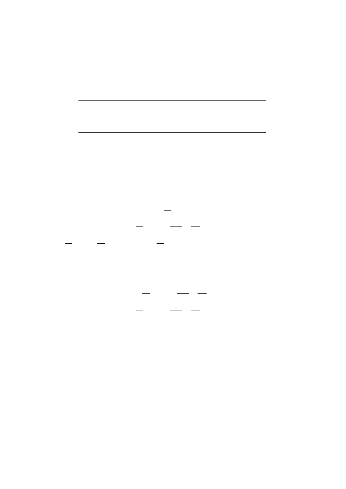
. By using Table 1, we can obtain the balance equations of mass, linear momentum,
and angular momentum.
Table 1. Volume densities, their supply and flux terms in the balance equations.
ψz f φ
ρ0ni(wi−vi)ρ0
ρvjρgjni(wi−vi)ρvjσij
ρ(sj+ejkl xkvl)ρ(`j+ejkl xkgl)ni(wi−vi)ρ(sj+ejkl xkvl)mij +ejkl xkσil
The domain may have its own velocity,
x•
i=wi
, independent on the velocity of the fluid
particle,
vi
. For a discussion of the balance equations in a control volume with the domain velocity,
we refer to [
55
,
56
]. This domain velocity can be chosen arbitrarily without affecting the underlying
physics. Herein we fix the domain by setting
wi=
0. We assume that initially the fluid rests,
vi(x
,
t=
0
) =
0, and it is a homogeneous material,
ρ(x
,
t=
0
) = const
. Moreover, we assume that the
flow is incompressible, i.e., the mass density remains constant in time,
∂ρ/∂t=
0. After utilizing the
Gauss–Ostrogradskiy theorem, we obtain
ZΩρ∂vi
∂xi
dv =0 , (5a)
ZΩρ∂vj
∂t−ρgj+ρ∂vivj
∂xi
−∂σij
∂xidv =0 , (5b)
ZΩρ∂sj
∂t+ρejklxk
∂vl
∂t−ρ`j−ρejkixkgi−∂
∂xi−viρ(sj+ejkl xkvl) + mij +ejkl xkσildv =0 , (5c)
where the spin density,
si
, its flux term (couple stress),
mij
, and its supply term,
`i
, they all vanish
for a non-polar medium like water (furnishing a symmetric stress). Then the angular momentum is
identical to the moment of (linear) momentum,
ZΩejkl xkρ∂vl
∂t−ρgl+ρ∂vivl
∂xi
−∂σil
∂xidv =0 , (6a)
ZΩρ∂vl
∂t−ρgl+ρ∂vivl
∂xi
−∂σil
∂xidv =0 , (6b)
hence, in analytical mechanics, we may neglect it. However, we observe this term as being important
for resolving numerical challenges.
We multiply the latter equations by an arbitrary test function with the same rank of the integrand,
i.e., Equation
(5a)
by a scalar, Equation
(5b)
by a vector, and Equation
(6b)
by a vector. Having an
arbitrary test function ensures that the global condition holds locally as well. According to the
Galerkin approach, we will choose the test functions from the same space as the unknowns,
viand p
.
Therefore, it is natural to use
δp
and
δvi
as possible test functions. As we need another vector as well,
we may choose
δvi
or even construct a vector by using gradient of
δp
. By utilizing the latter, we affect
the velocity distribution by the pressure gradient leading to an additional enforcement of the correct
pressure distribution. We know that several numerical problems start by computing the pressure
distribution wrongly and we circumvent such numerical instabilities by choosing
∂δp/∂xl
as the test
function for Equation
(6b)
—this particular choice is one of the key contributions of this work providing
stability and robustness to the computational method. A possible justification of this observation relies
on the restriction about the gradient of pressure, which may be interpreted as the missing condition for
the necessary numerical smoothness for pressure related to the LBB condition; however, we enforce it
by using an additional integral form instead of changing the order of shape functions. An analogous
Fluids 2019,4, 5 5 of 20
term multiplied by the mesh size is added in PSPG for the sake of a pressure stabilization. Herein we
use it in equal manner for every finite element independent of their size. Therefore, this formulation is
not called a stabilization since the same weak form is evaluated in each node with no dependence on
the mesh size.
We begin utilizing the discrete representations of continuous fields; but we omit a clear distinction
in the notation since we never use continuous and discrete functions together. We underline that the
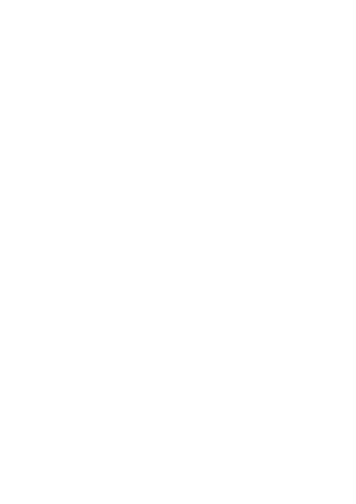
choice of the scalar test function is critical and we suggest to use
ZΩρ∂vi
∂xi
δpdv =0 , (7a)
ZΩρ∂vj
∂t−ρgj+ρ∂vivj
∂xi
−∂σij
∂xiδvjdv =0 , (7b)
ZΩρ∂vj
∂t−ρgj+ρ∂vivj
∂xi
−∂σij
∂xi∂δp
∂xj
dv =0 . (7c)
We refrain ourselves from inserting the mass balance,
∂vi/∂xi=
0, into the latter formulation.
In many implementations in the literature, as velocity divergence has to vanish (for incompressibility),
the term
∂vi/∂xi=
0 is inserted in Equation
(7b)
. Since this condition is tested by
δp
, we cannot
expect that it is fulfilled for the velocity distribution, thus, we choose to enforce it by testing with
δvj
in Equation
(7b)
. We stress that this particular choice improves the robustness of the numerical
implementation.
We solve the transient integral forms in discrete time slices with a time step
∆t
, this discretization
in time is established by using Euler backwards method resulting in
∂vi
∂t=vi−v0
i
∆t,(8)
where
v0
i
indicates the value from the last time step. This implicit method is stable (for real valued
problems) and easy to implement. We emphasize that the implementation is an implicit method since
we evaluate the derivative at the current time. Simply by using a Taylor series around the current time,
vi(t−∆t) = vi(t)−∆t∂vi
∂t+O(∆t2),(9)
and truncating after the linear term in
∆t
, we immediately obtain Equation
(8)
. As we neglect quadratic
time steps, we have to choose small time steps in the simulation in order to increase the accuracy of
the time discretization.
3. Generating the Weak Form
Integral forms in Equation
(7)
will be rewritten in the same unit such that we can sum them
up. First, we divide Equation
(7a)
by the mass density
ρ
and bring it to the unit of power.
Second, we undertake no changes in Equation
(7b)
as it is already in the unit of power. Third, we divide
Equation
(7c)
by the mass density and multiply it by the time step
∆t
and bring it also to the unit of
power. The choice of the unit, herein the unit of power, is arbitrary. Often the formulation is employed
in a dimensionless form generating the well-known Reynolds number.
We rewrite the constitutive equation,
σij =−pδij +τij
, by combining all terms with
dij
into
τij
.
The symmetric part of the velocity gradient,
dij
, thus the term
τij
already includes velocity’s first
derivative in space. As a consequence of the first derivative, we need to have a representation of the
velocity function, which is at least
C1
continuous. In the integral forms, we observe another space
derivative in
τij
leading to the restriction that a velocity approximation belonging to the class
C2
has to be implemented. This condition will be weakened by integrating by parts. We emphasize
that the integration by parts is applied only on the terms having (at least) second derivative of the
Loading more pages...