Simplified vortex methods to model wake vortex roll-up in real-time simulations for fuel-saving formation flight [original]

Vol.:(0123456789)

1 3

CEAS Aeronautical Journal (2022) 13:763–778

https://doi.org/10.1007/s13272-022-00587-1

ORIGINAL PAPER

Simplified vortex methods tomodel wake vortex roll‑up inreal‑time

simulations forfuel‑saving formation flight

HenrikSpark1 · RobertLuckner1

Received: 18 August 2021 / Revised: 25 April 2022 / Accepted: 28 April 2022 / Published online: 29 June 2022

Abstract

One possibility for reducing fuel consumption is to fly in the upwind field of the wake vortex generated by an aircraft that

is flying ahead. Migratory birds use this principle. Manually flying an aircraft at the point of optimal fuel reduction is not

suited for routine flight operations as the pilot workload is excessively high. Hence, an autopilot function has to carry out this

task. For designing the autopilot, a flight mechanical simulation with a wake vortex velocity model is required that has the

ability to calculate the vortex-induced velocity fields. This paper contributes to the choice of a real-time simulation method

for modelling vortex-induced velocities that the wake vortex of a leading aircraft generates and that the trailing aircraft shall

use during fuel-saving formation flight.Two different wake vortex velocity models are introduced and compared during

steady, horizontal flight. One model is based on the Lifting Line Method (LLM) and the other on the unsteady Vortex Lat-

tice Method (VLM). Both models are able to calculate the wake vortex roll-up phase for arbitrary lift distributions, whereas

the commonly used Single Horseshoe Vortex Model (SHVM) ignores the near-field roll up. The differences in the induced

upwind distribution and vortex filament position are analysed for coarse spatial and temporal discretisation that the real-time

constraint requires. Despite the more stringent simplifications of LLM, both methods yield similar filament positions and

similar velocity fields for the same discretisation of the lifting surfaces. Finally, the influence of the discretisation parameters

is discussed and parameter values are recommended for using VLM and LLM in real-time flight simulations.

Keywords Wake vortex modelling· Fuel saving formation flight· Real-time flight simulation· Vortex Lattice Method·

Lifting Line Method

List of symbols

b Wing span [m]

Vortex pair spacing [m]

Lift coefficient [–]

d𝐥

Discrete vortex filament segment [m]

H Altitude [m]

l(y) Chord length [m]

Core radius [m]

𝐫

Distance vector [m]

Vortex spacing parameter [m]

V Airspeed [m/s]

𝛼

Angle of attack [

◦

]

Circulation [

m2∕s

]

Γ0

Root circulation [

m2∕s

]

𝜌

Air density [

kg∕m3

]

Subscript/abbreviation

a Aerodynamic coordinate system

f Body coordinate system

ind Induced

W Wing

HTP Horizontal tailplane

TE Trailing edge

1 Introduction

Aviation has to noticeably reduce its environmental impact.

Innovative airframe and engine concepts as well as sus-

tainable aviation fuels shall contribute [1]. Also aircraft

operations shall be part of the solution [2]. Even though not

explicitly mentioned in Refs. [1, 2], it is long known that for-

mation flying techniques, inspired by migratory birds, have

the potential to significantly save energy. Transport aircraft

* Henrik Spark

[email protected]

1 Chair ofFlight Mechanics, Flight Control andAeroelasticity,

Institute ofAeronautics andAstronautics, Technical

University ofBerlin, Marchstr. 12, 10587Berlin,

Deutschland

764 H.Spark, R.Luckner

1 3

can use this technique as well. The Applied Vehicle Tech-

nology (AVT) Panel of the NATO Science and Technology

Organization (STO) has published a comprehensive over-

view on the state of the art of formation flight and the related

research activities including an extensive reference compi-

lation [3]. The overview addresses the history of energy-

saving formation flight, the physical principles, related tech-

nologies and systems, as well as operational aspects.

In a formation, the following aircraft can reduce its thrust

and hence its fuel consumption, when flying in the upwind

field of a wake vortex that a leading aircraft generates. So,

the trailing aircraft takes advantage of wake energy that

otherwise is left unused. The position for maximum fuel

savings in a vortex-induced velocity field is called sweet-

spot. For flying in the sweet-spot, the trailing aircraft has to

control its position relative to the leader. During long haul

flights, where the sweet-spot position has to be maintained

over many hours, formation flight needs to be automated.

This automation requires new autopilot functions. For the

development of such autopilot functions, a flight mechanical

model with a realistic wake vortex velocity model is needed

to simulate the vortex-induced forces and moments. Vortex

methods, as comprehensively described in Ref. [4], are used

for generation of vortex velocity fields. The research at the

TU Berlin aims at increasing the realism of formation flight

simulations by means of high-fidelity, real-time methods.

The objective of this paper is to evaluate the fidelity of real-

time methods for the calculation of the vortex velocity field.

Wieselberger [6] was the first who described the funda-

mental physics of formation flight by the vortex pair behind

a lifting surface. He calculated the upwind field by Biot

Savart’s Law. Schlichting [7] explained the resulting energy

savings by applying Aerodynamic Wing Theory. Hummel

[8] extended this approach to inhomogeneous formations.

In 1986, Beukenberg and Hummel demonstrated the theo-

retically explained energy savings by flight tests for the first

time [9, 10]. Further flight tests with different aircraft types

confirmed fuel savings up to 18%, for example in Ref. [11].

A simple vortex model that is commonly used for simula-

tions of formation flight and wake vortex encounters is the

Single Horseshoe Vortex Model (SHVM). It approximates

the wake vortex system by a pair of two straight vortices, see

Refs. [5] and [12]. This vortex model represents a rolled-up

vortex. It is valid from 15 up to 150 wing spans behind an

aircraft. Hence, it is not well suited to model the near field of

the wake that extends up to 15 wing spans behind the vortex

generating aircraft. As formation flight can be in within the

near field, modelling the vortex roll-up increases realism.

Sarpkaya [13] comprehensively reviews the computa-

tional methods that are developed in fluid mechanics to sim-

ulate and describe the characteristics of three-dimensional,

unsteady vortical flows. The application of those methods

to real-time flight simulator investigations is not straight

forward, as the real-time requirements on the computational

performance significantly differ from accuracy requirements

for fluid dynamic applications.

Fuel-saving formation flights are assumed to be carried

out when atmospheric turbulence is so low that decay and

deformation of the wake can be neglected for the envisioned

separation distances. However, to investigate cockpit pro-

cedures and pilot workload in real-time flight simulators,

vortex models are necessary for distances, where the vortex

roll-up is not completed (10 wing spans are 0.5 NM for an

80 m wing span aircraft like Airbus A380). Whereas the

computational-cheap SHVM can be used for formations with

separations above 15 wing spans, more accurate methods are

needed for closer distances.

For the investigation of vortex effects on a trailing air-

craft, very high accurate methods, like Large Eddy Simula-

tions (LES), have been applied, e.g. by Bieniek etal. [14].

There, the vortex flow field was pre-computed for a cer-

tain distance behind the generating aircraft and stored in

a “box”, from which the wind field can be used. If LES is

not available, LLM can be used in a similar manner—with

some loss of realism. However, such simulation techniques

require steady flight conditions. If the formation is manoeu-

vring, e.g. changing altitude or course, a pragmatic solution

to stay with the “box” technique by adapting the box loca-

tion and orientation in space was proposed by Kaden [15].

A superior approach would be to use methods, like LLM or

VLM that can online address the impact of the lift changes

of the vortex-generating aircraft and the impact on the wing.

However, in real-time flight simulations, available CPU per-

formance constrains the discretisation granularity. The moti-

vation for this paper was to prepare the online approach by

comparing LLM and VLM vortex models using very coarse

discretisation.

Research on vortex methods for wake vortex roll-up simu-

lations dates back to the 1930s [16]. Numerical problems

resulting from this approach and methods permitting their

resolution have coined a research area, see Refs. [17–19].

In addition to summing up the state of the art, Devoria and

Mohseni [19] describe the possibility of chaotic vortex tra-

jectories in roll-up simulations. As a solution to this prob-

lem, extensions to the roll-up methods are recommended.

The extensions can, for example, rediscretise the vortex

elements, see Ref. [20], or introduce specific procedures to

regulate the distortion of the Langrangian methods, see Refs.

[21, 22].

This paper compares two well-known methods for the

calculation of the vortex velocity field: the Lifting Line

Method (LLM) and an unsteady Vortex Lattice Method

(VLM). Extensions of the LLM or VLM, as proposed by

Refs. [20–22], are not considered here. The focus is on the

comparison of the unaugmented LLM and VLM calculation

schemes and their results. Only the core radius function is

765

Simplified vortex methods tomodel wake vortex roll‑up inreal‑time simulations forfuel‑saving…

1 3

introduced as smoothing parameter. The results of the LLM

and VLM formulations are compared to the SHVM.

LLM can be used for all distances behind aircraft. Kaden

implemented the LLM code that is used at TU Berlin and

in his work. He compared it to the simple SHVM, see Refs.

[5, 15]. A set of parameters for the LLM was optimised to

match the vortex-induced velocities in the far field, where

the roll-up is complete, with SHVM. The optimised param-

eters comprise the number of vortex filaments, the integra-

tion step size

Δt

, the core radius

and its regularisation

function. The calculation consists of two main steps: first, an

offline computation of the vortex particle field, and second,

the subsequent calculation of the vortex-induced velocities

at the follower’s position. Using simplifying assumptions,

the LLM’s second step, important for the formation flight

simulations, has real-time capability and is therefore cur-

rently used at TU Berlin.

Also at TU Berlin, Loftfield developed an unsteady Vor-

tex Lattice Method (VLM) for flight mechanical investiga-

tions at separated air flow as part of the project MoSS [23].

The unsteady VLM enables the calculation of wake vortex

roll-up behind manoeuvring aircraft. Less simplifications

in the VLM yield more realism compared to the LLM. But,

the VLM is computational expensive and the present for-

mulation is not suited for real-time application. Here, the

unsteady VLM is used. It is applied to a steady, horizontal

cruise flight scenario. A one kilometre long wake vortex

wind field is generated by an offline simulation. For the same

scenario, the wind field is calculated by the LLM. This is

achieved by flying the aircraft through planes and capturing

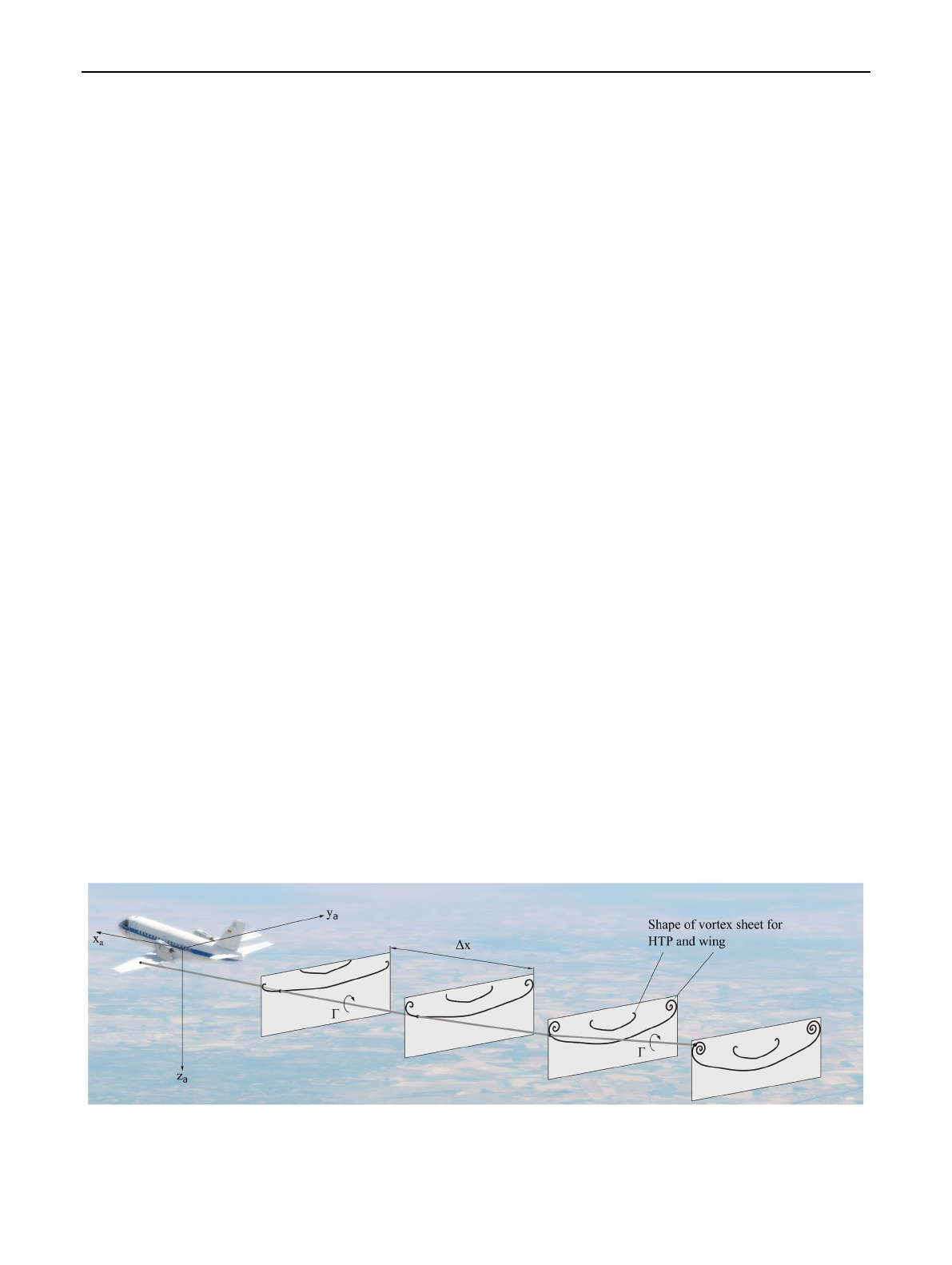
the wake properties at their locations, see Fig.1. Comparing

the results of both methods, the effect of the simplifications

made in the LLM is investigated.

For the comparison, the filament positions of the wake

vortices are analysed. The computed wind field data, result-

ing from all filament positions and circulations, are used

to identify the wake vortex axes. The axes represent the

wake vortex position. This position has to be known for

fuel-efficient formation flight. In addition to the position-

related comparison, the upwind areas in the wake vorti-

ces are compared. The vertical wind velocity maximum,

hence the maximum tangential velocity near the vortex

core, are related to the vortex-induced rolling moments, as

Bieniek has shown in Ref. [24]. Because the induced rolling

moments are important for the simulation of the following

aircraft, the vertical wind velocity maxima are used as a

substitute in our comparison.

The paper starts with the description of both wake vortex

methods LLM and VLM and the resulting models in Sect.2

addressing assumptions, differences, advantages and disad-

vantages. To enable a comparison, Sect.3 explains the meth-

odology to set up the models for a steady, horizontal flight

scenario. Section4 explains how the wake vortex axes are

identified. The identification method is used in Sect.5 for the

comparison of VLM and LLM results. Finally, an analysis of

the parameter set for this comparison is conducted in Sect.6.

2 Vortex filament methods

This section describes the methodologies behind LLM,

VLM and SHVM. SHVM is the reference as it is commonly

used in wake vortex simulations. The assumptions made by

the methods, the differences, advantages and disadvantages

of the LLM and VLM are explained.

LLM and VLM are Lagrangian methods, as described

in Refs. [4, 25, 26], tracing particles in a velocity field. The

particles are the edges of vortex filaments, which are shed

from the aircraft’s lifting surfaces. Using the Biot–Savart

law, see Sect.2.4, each filament induces a velocity on every

particle and therefore on every filament. The aircraft’s lift-

ing surfaces are modelled by vortex filaments, too. These

bound filaments also induce velocities, generating the flow

field around the lifting surfaces and influencing the wake

vortex roll-up. The mutual induced velocity of all vortex

filaments leads to a roll-up of the free filaments in the wake,

Fig. 1 Concept of the wake vortex roll-up simulation using grid planes according to Ref. [5]

766 H.Spark, R.Luckner

1 3

generating a rotational velocity field behind the left and right

wing of a leading aircraft. The induced velocity from the

opposing side induces the typical descent of the wake vortex.

In addition to calculating the induced velocity by the bound

and free filaments at the vortex filaments’ edges, the induced

velocity can be evaluated at arbitrary points to compute the

induced velocity fields.

Evaluation planes are placed behind an aircraft to calcu-

late and visualise the velocities induced by the vortex sheet

in grids. The evaluation planes can be arbitrarily placed.

They consist of a grid of particles. At the particle positions,

the local velocity is evaluated using the same operations as

for the free vortex filaments in the wake roll-up calculation.

The induced 3D velocity field is calculated from multiple

evaluation planes stacked in longitudinal

-direction.

Often, an elliptical lift distribution on the wing and tail-

plane is assumed for LLMs, see Refs. [5, 12, 27]. In this

paper, the regional airliner VFW 614 that is modelled at

TU Berlin’s research flight simulator is used as example.

Detailed geometric and aerodynamic data are available,

such as the exact geometry, wing twist and airfoil profiles.

Using those data, the elliptical distribution that was used

in previous projects is replaced by a lift distribution that is

calculated by the VLM. Thus, the wind field computation

starts with the VLM calculating the circulation at the lifting

surfaces (at the bound filaments). The following steps for the

wind field generation are equivalent in the VLM and LLM.

These steps are: computing the wake vortex roll-up, calculat-

ing the induced velocities at all particles in the evaluation

planes and saving the 3D wind field data.

2.1 Single horseshoe vortex model

The Single Horseshoe Vortex Model (SHVM) satisfyingly

represents the wake vortex velocity field after roll-up and it

is commonly utilised for that purpose, see Ref. [5]. Here, it

is used as reference for the LLM and VLM.

The SHVM consists of a bounded vortex at the wing

(its influence is commonly ignored) and two straight, free

counter-rotating vortices that extend behind the generating

aircraft to infinity. The circulation of the two straight vor-

tex lines is determined by the Kutta–Joukowski law using

the actual parameters of the leading aircraft. For a certain

vortex age, vortex decay can be considered by reducing the

circulation. In [5], Kaden defined the SHVM parameters

for cruise flight (weight of 17.4 tons, altitude of 6400 m

and airspeed of

140 m∕s

) for the VFW 614, assuming an

elliptical circulation distribution. The vortex spacing is

b0=

𝜋

∕4b=16.89 m

, circulation

Γ=114.42 m2∕s

, and

global core radius

rc=0.45 b=0.9675 m

In the following, the global core radius of the SHVM has

to be distinguished from the local core radius used to com-

pute the velocities induced by the discrete vortex filaments

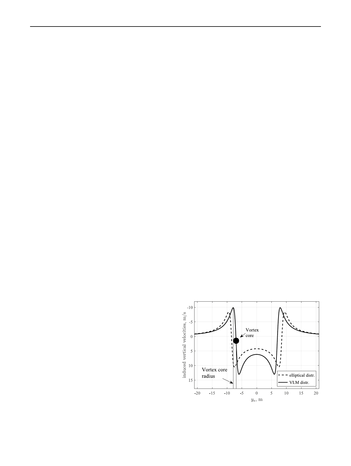
in LLM and VLM. Figure2 shows the resulting induced

vertical velocities for the elliptical circulation distribution

and for the distribution that is calculated by the VLM (for

discretisation 1, see Sect.3). In the VLM calculation, which

is used here, the values for aircraft mass, altitude and the

airspeed are the same as in [5] and yield

Γ=137.78 m2∕s

and a vortex spacing

b0=13.88 m

. The global core radius

is the same.

2.2 Lifting line method

The LLM calculates the roll-up in several steps that are

described in [5]. The wake vortex roll-up is calculated using

multiple calculation planes for the wake vortex roll-up cal-

culation, whereas the evaluation planes describe the 3D

wind field and define the vortex-induced wind field for an

aircraft flying through the planes. Both types of planes are

stacked in negative

-direction behind the aircraft in flight

direction, see Fig.1. The LLM represents lifting surfaces by

lifting lines. These lines hold a certain circulation distribu-

tion

Γ(y)

. The local circulation generally increases from a

lifting surface’s tip to its root. Following the Kutta–Jouk-

owski theorem, the lift is proportional to the circulation

air density

𝜌

and airspeed V [28]

The axis of the lifting lines are bound to the aircraft’s quarter

chord of the aerodynamic surfaces. Here, the bound vortex

filaments originate. The continuous circulation distribu-

tion

Γ(y)

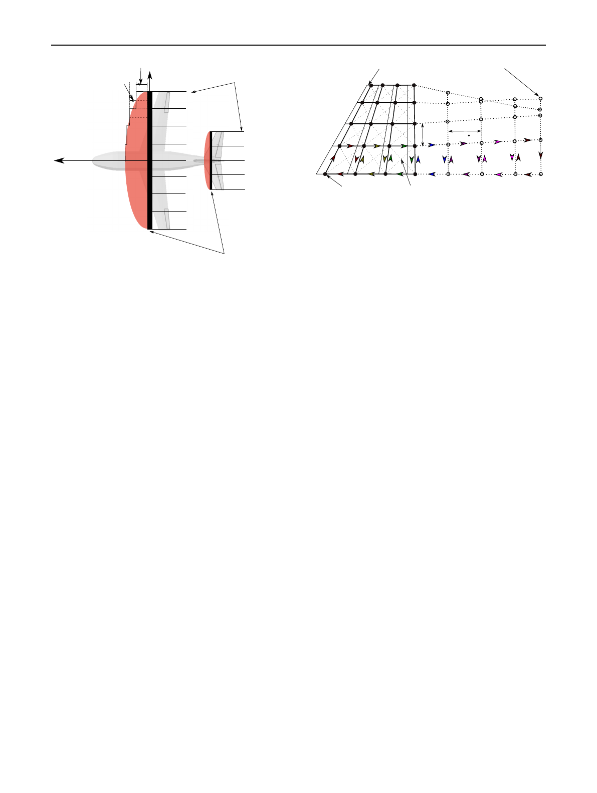
is replaced by the sum of the discrete circulations

ΔΓi

of the filaments with stepwise constant strength, see

Fig.3. Each discrete step in the bound circulation distribu-

tion produces a free vortex filament of the circulation

ΔΓi

see [29]. In other words, the discrete changes in the lifting

(2.1)

L=𝜌VΓ.

Fig. 2 Induced velocities of the SHVM with the VLM’s circulation

compared to the classical SHVM

767

Simplified vortex methods tomodel wake vortex roll‑up inreal‑time simulations forfuel‑saving…

1 3

line’s bound circulation determine the circulation of the free

wake vortex filaments.

The origin of the aerodynamic coordinate system (index

a) lies in the wing’s aerodynamic mean chord. The calcu-

lation planes span in

- and

-direction. The roll-up of

the free vortex filaments is calculated for each plane. The

time step size

Δt

is defined by the distance between those

planes,

Δt=Δxa∕V

. One can either assume the aircraft

to travel through the planes or assume that the planes are

following the aircraft in flight. For the previously intro-

duced evaluation planes, both points of view are equiva-

lent as the resultant wake age at each evaluation plane is

the same both ways when flying with a constant speed V.

The calculation planes are iteratively solved in the LLM

to calculate the wake shape. So, visualising the calculation

planes behind the aircraft and extending the wake shape in

each time step to the next gate is preferred. Another cal-

culation plane is added each time step to extend the wake

shape. The iterative calculation starts from the position of

the lifting lines and employs the forward Euler integration

method. In each calculation plane, the vortex filaments are

assumed to be straight and aligned with the

-axis. By

this approximation, the induced velocity in

-direction

vanishes and the roll-up is simplified, see Ref. [5]. So,

the LLM only uses the preceding calculation plane that

contains the last position of the free filaments to compute

the next position of the free filaments. The influence of

the bound filaments is considered, but it vanishes down-

stream. By using this approximation instead of calculating

the induced velocities from streaklines, the algorithm time

complexity of the calculation decreases.

As a result of this scheme, the runtime of the LLM scales

linear with the number of computation planes. Thus, it scales

linear with the wake vortex length. The runtime scales quad-

ratically with the number of vortex filaments, as all vortex

filaments interact. However, a disadvantage of LLM is, that

the lifting line’s circulation distribution has to be prescribed,

considering the necessary total lift of the aircraft. This can

either be done by assuming an elliptical distribution or, as in

this paper, by calculating the distribution for example with

the VLM.

2.3 Vortex lattice method

The unsteady Vortex Lattice Method (VLM) uses a lat-

tice of vortex filaments to represent the lifting surfaces and

the wake, as Fig.4 shows. Each lattice consists of indi-

vidual vortex rings, each vortex ring comprises four vortex

filaments.

Panels model the aircraft’s lifting surface geometry, as

described in Sect.3. Based on the panel position and the

convention to place the vortex rings’ leading segments at

the panels’ quarter chord [28], the vortex lattice geometry

is derived accordingly, see Fig.4. Each vortex ring has the

same oriented circulation

Γij

(circulation of panel i at sec-

tion j) for all four filaments of the ring, see Ref. [28]. The

vortex rings placed on the panel geometry are bound to that

geometry. Their circulation

Γij

is calculated so a no-flow-

through condition is reached at the collocation points. The

collocation points are placed at the centre of the vortex rings,

therefore at three quarter of the panels chord. The condition

that no flow passes through surfaces causes a tangential air-

flow over the lifting surfaces.

The free vortex rings representing the wake are gener-

ated at the lifting surfaces’ trailing edges and move with

their individual local velocity. Obeying the Helmholtz

theorems and the conservation of circulation [30], the cir-

culation of the free vortex rings is bound to the filaments

bound vortex filaments

free vortex filaments

ΔΓ2ΔΓ1

ΔΓ1

ΔΓ2

Fig. 3 Schematic of free vortex filaments origination at unswept lift-

ing lines

panel geometry

Γ1,1

bound vortex corner point

free vortex corner point

XXX

collocation point

Γ2,1 Γ3,1 Γw,1,1 Γw,2,1 Γw,3,1 Γw,4,1

Δx

Δy =Δt V

Fig. 4 Vortex lattice formed by four filaments per vortex ring,

adapted from [28] and [23]

Loading more pages...