Stability analysis of the Iraqi GNSS stations [original]

J. Appl. Geodesy 2022; aop

Sattar Isawi*, Harald Schuh, Benjamin Männel, and Pierre Sakic

Stability analysis of the Iraqi GNSS stations

https://doi.org/10.1515/jag-2022-0001

Received January 9, 2022; accepted February 20, 2022

Abstract: The Iraqi GNSS network was installed in 2005

with help from the USA and UK. The network consists of

seven GNSS stations distributed across Iraq. The network

GNSS data have been comprehensively analyzed in this

study; this, in turn, allowed us to assess the impact of var-

ious geophysical phenomena (e. g., tectonic plate motion

and Earthquakes) on its positional accuracy, stability, and

validity over time. We processed daily GPS data, spanning

over more than five years. The Earth Parameter and Or-

bit System software (EPOS.P8), developed by the German

Geoscience Research Center (GFZ), was used for data pro-

cessing by adopting the Precise Point Positioning (PPP)

strategy. The stacked time series of stations coordinates

was analyzed after estimating all modeled parameters of

deterministic and stochastic parts using the least-squares

technique. The study confirmed a slight impact of the re-

cent M 7.3 Earthquake on the Iraqi GNSS stations and con-

cluded that the stations are stable over the study period

(2013 up to 2018) and that the GNSS stations represent the

movement of the Arabian plate.

Keywords: CORS, time series analysis, power-law noise,

IGRS

1 Introduction

The crucial part of national infrastructure is establishing

an accurate spatial reference system that can be realized

by a reliable geodetic network of permanent control sta-

tions. These stations are referenced to a well-defined coor-

*Corresponding author: Sattar Isawi, Technische Universität Berlin,

Institute of Geodesy and Geoinformation Science, Strasse des 17.

Juni 135, 10623 Berlin, Germany, e-mail:

sattar.mb.isaw[email protected]u-berlin.de

Harald Schuh, Technische Universität Berlin, Institute of Geodesy

and Geoinformation Science, Strasse des 17. Juni 135, 10623 Berlin,

Germany; and GFZ German Research Centre for Geosciences,

Department of Geodesy, Telegrafenberg, 14473 Potsdam, Germany,

e-mail: harald.schuh@gfz-potsdam.de, ORCID:

https://orcid.org/0000-0001-5443-0370

Benjamin Männel, Pierre Sakic, GFZ German Research Centre for

Geosciences, Department of Geodesy, Telegrafenberg, 14473

Potsdam, Germany, e-mails: benjamin.maennel@gfz-potsdam.de,

pierre.sakic@gfz-potsdam.de, ORCID:

https://orcid.org/0000-0003-2938-1356 (B. Männel),

https://orcid.org/0000-0003-1770-0532 (P. Sakic)

dinate system to be the backbone of the nation’s geospatial

system (e. g., geodatabase and mapping systems).

Iraq followed this approach after the war in 2003

because reconstruction demanded implementing major

engineering projects. Moreover, the implementation of

these projects needs a stable and reliable geodetic basis.

Therefore, in 2005, Iraq established a new geodetic refer-

ence system called the Iraqi Geospatial Reference System

(IGRS). Since the establishment of IGRS, all new Iraqi en-

gineering projects and mapping systems were based on

it, specifically Oil & Gas, Transportation, Electrics, and

Agricultural projects. IGRS realized as a coincidence with

ITRF2000 at epoch 1997.0 but anchored to the Arabian

plate by five permanent GNSS stations [32]. In principle,

IGRS represents a snapshot of the Arabian plate’s dynamic

on which Iraq lies. Furthermore, IGRS is a dynamic ref-

erence frame that continuously moves with the Arabian

plate motion [10]. Besides, Iraq locates at the boundary be-

tween two different tectonic plates, Arabian and Eurasian

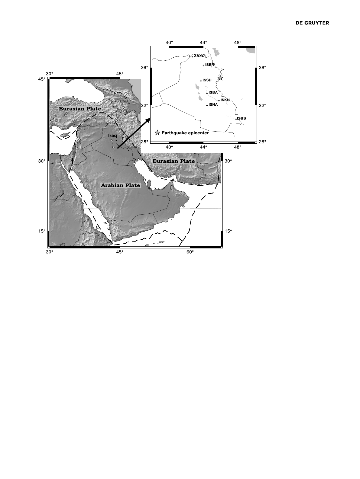
plates (Fig. 1). This area is deformable and continuously

unstable, as shown by several Earthquakes, for exam-

ple M 7.3 Iraq – Iran border earthquake on November 12,

2017 [26]. Quantifying the influence of such geophysical

processes on the stability of the Iraqi permanent GNSS sta-

tions necessitates an in-depth and comprehensive study

because of its significant impact on the present and future

geodetic surveying in Iraq.

The remarkable development of space geodetic tech-

niques (e. g., Global Navigation Satellite Systems GNSS)

made it easy to obtain continuous 3D positions for points

on Earth’s surface for very long periods of up to many

years. The obtained positions are characterized by suffi-

cient accuracy to monitor the GNSS station’s antenna posi-

tion change over time. This change indirectly refers to var-

ious physical processes in the Earth system (e. g., tectonic

plate motion).

Based on this proposition, several researchers stud-

ied the movement of the Arabian plate by adopting space

geodetic techniques. For example, [3] studied the Arabian

plate motion by estimating the Riyadh SLR station’s posi-

tion and velocity. Laser-ranging observations of 14 years

from 20 SLR stations to LAGEOS-1 and LAGEOS-2 have

been analyzed in this study. They concluded that the Ara-

bian plate is countering a north-east motion with an an-

nual linear rate of 42.9 mm/year. [11] processed ten years

of daily GPS data from two Iraqi GNSS stations. ISER, lo-

cated in Erbil, and ISNA, located in Najaf. The GITSA anal-

License.

2| S. Isawi et al., Stability analysis of the Iraqi GNSS stations

Figure 1: The spatial distribution of the Iraqi GNSS stations. The black dashed lines are the boundary of tectonic plates. The star symbol

represents the epicentre location of the M 7.3 Earthquake that hits Iraq – Iran border on November 12, 2017.

ysis software was used in this study to build up and ana-

lyze the time series of station coordinates. The study con-

cluded that the estimated velocity vectors for the ana-

lyzed stations were 38 mm/year and 40 mm/year, respec-

tively.

The estimation of linear rate (mainly driven by plate

motion) is the main focus of these studies. However, this

estimation needs an improvement to the adopted func-

tional model. The periodic effects (e. g., annual and semi-

annual deformation), sudden effects (e. g., offset due to

antenna change or co-seismic deformation), or even post-

seismic deformation have to be modeled and extracted

from the time series signal [4]. Although all common de-

terministic parts would be modeled for the time series, dif-

ferent noise sources are still present in its signal due to

satellite orbit error, atmospheric delays, and clock insta-

bility. On the other hand, the assumption that the only

white noise (uncorrelated noise) contributes to the noise

model will lead to underestimated uncertainty of linear ve-

locities by factors from three to six times [33], or even five

to 11 times [20].

The Iraqi GNSS stations will be extensively analyzed

in this study to assess the impact of various geophysical

processes (e. g., tectonic plate motion and Earthquakes) on

their accuracy, stability, and validity over the study period.

The determination of coordinate time series characteris-

tics (trend, annual signals, offsets, and spectra) will be fur-

ther described and discussed. Besides, this study will in-

vestigate the potential contribution of different noise types

(e. g., power-law noise) to the noise model. A Matlab code

comprises functions written to implement this study in

both the frequency and time domain.

2 Data

Five continuously operating GNSS reference stations have

been selected out of seven Iraqi GNSS stations for this

S. Isawi et al., Stability analysis of the Iraqi GNSS stations | 3

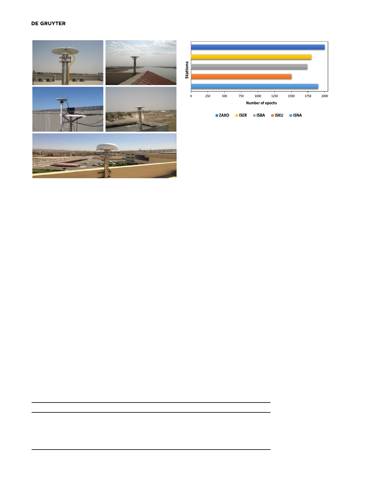
Figure 2: GPS antennas attached to the monuments. ISER, ISKU (top)

and ISBA, ISNA (middle), and ZAXO station (bottom). Source NGS at

https://www.ngs.noaa.gov/.

study. The selected GNSS stations are ISNA, ISKU, ISBA,

ISER, and ZAXO. ISBS and ISSD stations were excluded be-

cause both of them were non-operational during the inves-

tigated period. The spatial distribution of the Iraqi GNSS

stations is shown in Fig. (1). All selected GNSS stations

were equipped with dual-frequency GNSS receivers as well

as geodetic antenna types. However, all of them have non-

geodetic monuments because of the antennas mounted on

top of buildings (Fig. 2). Station ISBA is part of the Inter-

national GNSS Service (IGS) network [12], whereas the re-

maining stations are a part of the National Geodetic Survey

(NGS) global network.

The daily observation (raw data) of all GNSS stations

were downloaded from the NGS public archive at ftp://

geodesy.noaa.gov/cors/rinex/. The number of daily obser-

vation files for each station is shown in Fig. (3). The GNSS

station’s meta-data (log files) needed to track the station

history were also obtained from the NGS database system

(Table 1). The data included a comprehensive record of sta-

Figure 3: Number of daily observation files per station.

tion firmware and hardware changes (e. g., GNSS receiver

and antenna type). A pre knowledge in station history is

required in this study because the change in station hard-

ware and software could lead to offsets in the position time

series [27].

2.1 GPS daily solutions

The software package EPOS.P8, developed at GFZ, was

used to process the GPS data. Satellite orbits, clock cor-

rections, and Earth Orientation Parameters (EOP) were

provided by a GFZ internal reprocessing based on the

operational final solution [18]. The products were given

in the IGS14 reference frame. Our final solution of the

GPS daily coordinates for each station was estimated fol-

lowing the Precise-Point-Positioning (PPP) methodology

adopted in GFZ AC. The processing details (Table 11) and

the flow diagram (Fig. 8) of PPP processing are shown in

Appendix A.

3 Methods

Firstly, the 3-D Cartesian coordinates Xi,Yi, and Ziob-

tained from GNSS data processing were transformed into

topocentric North, East, and Up. The coordinate trans-

formation from the right-hand system Earth Centered

Table 1: Log files information of selected GNSS Stations.

ISNA ISKU ISBA ISER ZAXO

City Najaf Kut Baghdad Erbil Dohuk

Sat. System GPS+GLO GPS+GLO GPS+GLO GPS+GLO GPS

GPS Receiver TRM NETR9 TRM TRM NETR5 TRM NETR5 TPS NET-G3A

Ant. Type TRM57971 TRM57971 TRM41249 TRM57971 TPSCR.G5

Monum. Desc. Tribr. adap. Trib. adap. Trib. adap. Trib. adap. Trib. adap.

4| S. Isawi et al., Stability analysis of the Iraqi GNSS stations

Earth Fixed (ECEF) into the topocentric left-hand system

has been implemented according to [24]. The variance-

covariance matrix SXYZ of GNSS daily solutions have also

been transformed into the topocentric system by applying

a variance-covariance propagation law [25].

3.1 Functional model

The time series for individual topocentric components

(North, East, and Up) was built up based on the GNSS daily

solutions ytiat uniformly spaced time ti(i=1,...,n, where n

is the number of daily solutions). The stacked time series

have been modeled (approximated) as the sum of deter-

ministic parts, by considering the initial site position x0,

and linear rate vx(interpreted as the GNSS station veloc-

ity), as well as the periodic signals of annual and semi-

annual motion. The functional model reads:

yti=x0+vxti+asin(2πti)+bcos(2πti)+csin(4πti)

+dcos(4πti)+εi(1)

with aand bare the coefficients of the annual periodic

motion, while cand dare the coefficients of semi annual

motion. When there are in addition moffsets (jumps) in

the coordinate time series, the functional model can be ex-

panded to [6]:

yti=x0+vxti+asin(2πti)+bcos(2πti)+csin(4πti)

+dcos(4πti)+m

∑

j=1

fjh(ti−tfj)+εi(2)

where fjis the offset’s magnitude, tfj is the offset’s epoch

with hdenoting the Heaviside function, and εis the model

error. With apriori known offset epochs tfj, the linear model

of observation equations in Eq. (2) is solved using the least-

squares method:



x=(ATSyy−1A)−1ATSyy−1y,(3)

where the vector of adjusted unknowns 

xconsists of the

following parameters:



x=[

x0

vx

a

b

c

d

f]T,(4)

Syy is the variance-covariance matrix of the observation

vector y,

y=[yt1,...,ytn]T,(5)

and, the design matrix Ais given as:

A=[[[[

1t1sin(2πt1)cos(2πt1)sin(4πt1)cos(4πt1)h(t1−tfn)

1tnsin(2πtn)cos(2πtn)sin(4πtn)cos(4πtn)h(tn−tfm)]]]]

(6)

Table 2: Summary of coordinate data.

Site Data Start epoch End epoch Outliers

# # %

ISBA

N 1743 2013.00 2018.99 134 7.6

E 1743 2013.00 2018.99 116 6.6

U 1743 2013.00 2018.99 145 8.3

ISNA

N 1327 2013.00 2018.99 89 6.7

E 1327 2013.00 2018.99 88 6.6

U 1327 2013.00 2018.99 51 3.8

ISKU

N 1591 2013.00 2018.99 70 4.3

E 1591 2013.00 2018.99 78 4.9

U 1591 2013.00 2018.99 100 6.2

ISER

N 1837 2013.00 2018.99 284 15.4

E 1837 2013.00 2018.99 267 14.5

U 1837 2013.00 2018.99 155 8.4

ZAXO

N 1090 2015.00 2018.99 110 10

E 1090 2015.00 2018.99 69 6.3

U 1090 2015.00 2018.99 65 5.9

3.2 Outlier detection and removal

Outliers have been detected and removed from each co-

ordinate time series during the preliminary model fitting.

The median and interquartile range approach [21] were im-

plemented in this study. The median and IQR statistics are

calculated for the residuals on a sliding window of one

year centered on each time series element to consider the

gradual decrease in the data variance associated with the

increase in the time series length. Outliers were defined as

having:

|vi−median|>1.5×IQR (7)

where IQR defines the middle 50 % of the sample data, and

viis the ith least square residual.

Summary of removed outliers for each station time se-

ries is presented in Table (2).

4 Noise characteristics and

analysis

As with many other geophysical phenomena, noise in co-

ordinate time series can be described as a power law pro-

cess of the form [2, 16]:

S. Isawi et al., Stability analysis of the Iraqi GNSS stations | 5

Pv(f)=P0(f

f0)k

(8)

where fis the temporal frequency, P0and f0are normal-

izing constants, and kis the spectral index that defines a

slope of the best fit line to the spectra presented in log-log

space [33]. A smaller spectral index implies a more corre-

lated process and a more relative power at lower frequen-

cies. Therefore such a natural process is characterized by

negative indices [13]. According to [17], the spectral index

of different geophysical phenomena is classified into two

groups. The first group is called fractional Brownian mo-

tion with spectral index −3<k< −1. The noise processes

in this interval are non-stationary including random walk

with k= −2 or(Px∝1/f2), while the second group termed

fractional Gaussian with spectral index −1<k< +1, where

the noise processes in this interval are stationary (inde-

pendent of time) including the special case of uncorrelated

white noise with k=0 or (Px∝1/f0). The special case

k= −1 or (Px∝1/f1) is known as “flicker noise”. Plenty

of studies showed that the spectral index has particular

importance because it is a good indicator for characteriz-

ing the noise source [14, 22]. Based on the preceding, it is

necessary to study the post-fit residuals in-depth to decide

which colored (correlated) noise type has to be considered

in the noise model.

Two approaches are described in the literature to clas-

sify and quantify noise in the coordinate time series. The

first approach’s implementation relies on time series anal-

ysis in the frequency domain (spectral analysis). In con-

trast, the second one relies on the time series analysis in

the time domain. In this study, we restricted ourselves to

the second approach, but in addition, only estimating the

spectral index in the frequency domain.

4.1 Noise analysis

The time series signal and its noise do not behave in the

same way when transformed and plotted as a power spec-

trum. This property can be of great benefit for noise anal-

ysis in the frequency domain. Based on this concept, the

time series of post-fit residuals have been transformed into

the frequency domain for further analysis.

Unfortunately, equipment malfunction, interruptions

in the communications network, or even outlier removal

lead to missing data in the coordinate time series. There-

fore, a Lomb-Scargle periodogram introduced by [15] and

used by [33] has been applied to solve this issue.

According to [33], the time series of post-fit residuals

must be long enough and comprise data with a range of fre-

quencies that make the power spectra well approximated.

Hence, from the practical aspect, the spectral index of the

power-law process can be estimated by fitting a straight

line to these frequencies to avoid biasing the regression es-

timate with the predominance of white noise at high fre-

quencies and decreasing the impact of outliers at lower

frequencies. The functional model of power-law process in

Eq. (8) can be reformulated as:

Pvi(f)=P0

f0kfi

k(9)

substitution leads to

W0=P0

f0k(10)

Taking the log of both sides yields

log(Pvi(f)) =log(W0)+klog(fi)(11)

where all parameters are defined as in Eq. (8). To estimate

the slope of the fitted line (spectral index k) to the spec-

tra at log-log space, the least-squares method was used.

Therefore, Eq. (3) has been applied with the design matrix

of the form:

A=[[[[[[[[[[

1 log(f1)

1 log(f2)

. .

1 log(fN)

]]]]]]]]]]

(12)

The spectral index has been estimated for each time se-

ries. The proper noise model was founded on a combina-

tion of white and flicker noises. Since the amplitudes of

both noises have to be known in the adopted noise model,

the contribution for each noise has been estimated in this

study using the Maximum likelihood method presented

in [30]. In this approach, the amplitudes (variances) were

estimated by explicitly maximizing the likelihood function

for the total variance σ2

σ2=

vTC−1

N(13)

where C is the covariance matrix of post-fit residuals, N is

the number of daily solutions, and 

v is the vector of post-

fit residuals. According to [30], the covariance matrix C can

be decomposed into two components with amplitudes σ2

and σ2

kbeing the variance of white and power-law noises

respectively such that:

C=σ2

wIw+σ2

kJk(14)

Loading more pages...