Time domain modelling and stability analysis of complex thermoacoustic systems [original]

657

Time domain modelling and stability analysis of

complex thermoacoustic systems†

M R Bothien∗,J P Moeck, A Lacarelle,and C O Paschereit

Institute of Fluid Dynamics and Engineering Acoustics (Hermann-Föttinger-Institute), Technical University Berlin,

Berlin, Germany

The manuscript was received on 31 October 2006 and was accepted after revision for publication on 11 April 2007.

DOI: 10.1243/09576509JPE384

Abstract: A methodology allowing for a modular setup of complex acoustic systems is developed.

The transfer behaviour of the individual subsystems is formulated in time domain. Subsystem

descriptions can be obtained by analytical considerations, numerical methods, or experimental

data. Once the complex subsystems have been characterized experimentally, changes in sys-

tem geometry can be implemented easily by exchanging or adding subsystems. To validate the

modelling approach, experiments are conducted in an acoustic test rig with a combustor-type

geometry. Results are compared to predictions from the model, demonstrating accuracy in fre-

quency and time domain. Application to thermoacoustic instabilities arising in lean-premixed

combustion is given.The influence of a modified fuel distribution on an unstable operating point

of a lean-premixed combustor is studied and validated with experimental data. Additionally, a

study on the parameters governing the flame transfer function is performed to generate a stability

map of a model combustor. An advantage of the state-space approach is that stability of a ther-

moacoustic system can be determined by simply solving a matrix eigenvalue problem. This is in

strong contrast to the traditional approach, where the complete model is formulated in frequency

domain with infinite-dimensional transfer functions. The time domain approach is based on the

methodology presented by Schuermans et al. [1]. In contrast to their work, however, subsystems

are not obtained from modal expansions but are characterized by using system identification

techniques. Additionally, accuracy of the time domain model is verified by experiments.

Keywords: stability analysis, state-space system, thermoacoustics, time domain simulation

1 INTRODUCTION

As emission levels for modern gas turbines become

more and more restrictive, the gas turbine industry

stays abreast of changes by using lean-premixed com-

bustion. However, the leaner a combustion system

operates the more it is prone to suddenly occur-

ring large pressure oscillations. These so-called ther-

moacoustic instabilities arise from the interaction of

∗Corresponding author: Institute of Fluid Dynamics and Engineer-

ing Acoustics (Hermann-Föttinger-Institute), Technical University

Berlin, Müller-Breslau-Straße 8, 10623 Berlin, Germany. email:

mirko[email protected]

†Extended version of a paper originally presented at the 2006 Con-

ference on Modelling Fluid Flow (CMFF’06),Budapest University of

Technology and Economics, 6–9 Sepetember 2006.

unsteady heat release and the acoustic field in the

engine. If the two mechanisms constructively inter-

fere, high amplitude pressure pulsations occur, which

have a detrimental effect on the combustion pro-

cess [2]. Among others, Dowling and Hubbard [3]

expressed this fact in terms of an acoustic energy

equation, which states that perturbations grow if their

net energy gain from the combustion–acoustic inter-

action is greater than their losses across the system

boundaries and due to dissipation.

Thermoacoustic instabilities are a major issue in gas

turbines – both in stationary and aerospace applica-

tions but also in boilers and furnaces [2,4,5]. Strong

pressure oscillations cause higher emissions of pollu-

tants (NOxand CO), decrease the engine performance

and significantly increase the noise level. If the fluctu-

ations are high enough, they can even cause structural

damage [2,6,7].

JPE384 ©IMechE 2007 Proc. IMechE Vol. 221 Part A: J. Power and Energy

658 M R Bothien,J P Moeck,A Lacarelle,andCOPaschereit

To predict unreliable and unsafe operation, it is

necessary to describe how the system’s acoustic field

couples with the heat release. A model of the acous-

tic properties, supplemented by information on the

flame response, allows for prediction and control

of combustion instabilities. Thus, maintenance rates

can be extended and the operating process can be

improved. Furthermore, a model can also be used to

formulate design constraints to new burner develop-

ments.

As full-scale engine tests are extremely costly and

time-consuming, detailed investigations of thermoa-

coustic phenomena are commonly conducted in sin-

gle burner test rigs. Due to the high complexity of

geometry and interaction mechanisms in combustion

systems,a comprehensivedescriptionoftheiracoustic

field is cumbersome [1]. Although detailed numer-

ical simulations (taking into account reaction, flow,

and acoustics) were shown to be able to accurately

calculate the thermoacoustic interaction mechanisms

in single burner configurations [8], time expense,

and computing power requirements are very high.

Schuermans et al. [9] decreased the computational

effort by coupling low-order acoustic models, repre-

senting complex impedance boundary conditions, to a

computational fluid dynamics (CFD) solver. Especially

if stability has to be assessed for a high number of

parameter combinations (as shown in section 5), the

use of a CFD code is not practicable. Moreover, as a

CFD simulation is only able to observe the dominant

mode of the instability, it is usually not possible to

assess more linearly unstable modes [10]. Additionally,

marginally stable modes cannot be detected, which

is in contrast to the network approach described in

the following. Sattelmayer and Polifke [11,12] stated

that it is extremely difficult to derive suitable mea-

sures to improve the system stability using results

of large eddy simulation (LES) calculations, although

these are able to give detailed information on the

periodic reacting flow. Therefore, methods based on

analytical modelling will remain the most appropri-

ate stability assessment tool in the relatively near

future.

One further step to reduce computational effort is

to use low-order models to describe the whole com-

bustion system. The common approach is to divide

the total system into several subsystems, which are

described by transfer functions accounting for plane

wave propagation. Connection of these subsystems

results in a low-order representation of the total

system’s acoustic properties. The network approach

has the main advantages that information about

the system’s acoustics and insight into the phys-

ical processes can be obtained very quickly [13],

which is of major importance in early design phases.

Furthermore, changes in geometry or setup, as

for example the performance of different burners,

can easily be implemented in the model by sim-

ply exchanging a subsystem. Due to this modular

setup, it is possible to incorporate an experimen-

tally determined flame transfer function in the model.

The flame–acoustic interaction is crucial for the sta-

bility of thermoacoustic systems and it is far from

trivial to represent the linear flame response accu-

rately in a CFD computation. A drawback of this

approach is the limitation to plane wave acoustics.

To overcome this problem, multi-dimensional mod-

els have to be considered. Evesque and Polifke [13]

set up a two-dimensional low-order network, which

was validated against a three-dimensional finite ele-

ment method (FEM) solver showing good agree-

ment.

Traditionally, stability analysis of thermoacoustic

systems is accomplished by setting up a low-order

network model, which is then investigated in the fre-

quency domain. This is either done by solving the

system’s dispersion relation [14,15], or by graphical

methods (Nyquist plots) as described by Sattelmayer

and Polifke [11,12]. Both the graphical approach and

finding the roots of the dispersion relation are gen-

erally not trivial but rather time-consuming tasks,

especially if stability maps have to be generated [16].

In contrast to the traditional frequency domain

approach, another procedure is followed here, by

modelling the acoustic properties of the system in the

time domain. Therefore, all subsystems are character-

ized in state-space form. For the resulting state-space

network system, only a matrix eigenvalue problem has

to be solved to perform a stability analysis, which is

numerically straightforward.Schuermansetal. [7] also

described the system in state-space form, however,

they used modal expansion techniques to describe the

individual subsystems.

Once a model for the thermoacoustic proper-

ties of the combustion system is at hand, control

strategies can be implemented to suppress the feed-

back cycle. These strategies can either be passive by

implementing changes in the combustor geometry or

introduction of damping devices (e.g. Helmholtz or

λ/4-resonators) [17,18], or active by means of open-

or closed-loop control [3,19].

The remaining parts are structured as follows: sec-

tions 2 and 3 deal with the characterization of the sub-

systems in state-space form. The modelling approach

is validated against experimental data in section 4.

Application to thermoacoustic stability analysis is

then given in section 5. Here, results from frequency

domain and state-space calculations are also com-

pared. In section 6, a simulation model is used to

predict the stabilizing influence of a modified fuel

distribution in an experimental lean-premixed com-

bustor.

Proc. IMechE Vol. 221 Part A: J. Power and Energy JPE384 ©IMechE 2007

Modelling and analysis of complex thermoacoustic systems 659

2 STATE-SPACE REPRESENTATION OF ACOUSTIC

SUBSYSTEMS

As in the frequency domain transfer matrix approach

[20], it is assumed that only plane waves propagate

between two subsystems. This assumption is valid for

elements that are coupled via ducts, for which the fre-

quencies considered are below the cut-on frequency of

the first non-planar mode. Neglecting entropy waves,

this results in two degrees of freedom for all coupling

planes. The variables accounting for that can be either

acoustic pressure pand velocity vor the Riemann

invariants of the plane wave field, denoted here with f

and gfor downstream and upstream travelling waves,

respectively. The primitive variables are related to

the Riemann invariants by p=f+gand v=f−g.

Here (as in the following), the acoustic pressure has

been scaled with the characteristic impedance ρc, the

product of density and speed of sound.

Subsequently, acoustic systems are characterized

using the scattering form, i.e. the f-wave upstream

and the g-wave downstream are treated as inputs

and, accordingly, the f-wave downstream and the

g-wave upstream are obtained as outputs.The generic

acoustic element in state-space form can then be

written as

x=Ax+Bfu

gd

fd

gu=Cx+Dfu

gd

(1)

where subscripts u and d denote upstream and down-

stream positions, respectively. A,B,C, and Dare

time-invariant N×N,N×2, 2 ×N, and 2 ×2 matri-

ces, respectively, and xis the N-dimensional state

vector. The dimension of the state depends on the

acoustic subsystem to be characterized and has to

be chosen sufficiently large so that the system’s fre-

quency response is represented with acceptable accu-

racy in the frequency range considered. An inlet or exit

boundary condition can be written similar to equation

(1) as a single input single output (SISO) system.

3 SUBSYSTEM CHARACTERIZATION

The modular setup allows for different ways of describ-

ing the subsystems, i.e. by analytical considerations,

experimental data, or numerical methods (e.g. using

FEM [21]). The subsystems’ transfer functions relate

the incoming and outgoing acoustic waves. Usually,

acoustic subsystem characterization based on FEM

computations or experiments results in frequency

domain data. In the frequency domain the rela-

tion of the Riemann invariants is represented by the

scattering matrix S

fd

gu=S11 S12

S21 S22fu

gd(2)

where the elements Sij are complex-valued functions

of frequency.

Once a subsystem’s acoustic transfer function is

given in the frequency-dependent form, equation (2),

it can easily be transformed into the corresponding

state-space form (equation (1)). The elements of the

matrices of this state-space realization depend on how

the system’s state-space variables are defined. The

same input-output behaviour can be obtained from

different definitions of the system’s state variables. If

these variables are determined from the poles of a

partial fraction expansion of the elements Sij, which

is mostly the case in this article, the system matrix A

(equation (1)) assumes the so-called Jordan canonical

form. The diagonal elements then comprise the poles

of the partial fraction expansion. Detailed informa-

tion on how this and other state-space formulations

can be obtained from a transfer function in frequency

domain can be found in reference [22]. In the follow-

ing sections 4 and 5, more information on the specific

form ofthetransfer functionofeachindividual subsys-

tem is given. Here, either the scattering matrix, transfer

function, or state-space form is chosen, depending on

which formulation is more descriptive.

3.1 Analytical description

The description of elements with simple geome-

tries (e.g. ducts) is straightforward. Neglecting sound

absorption at the walls and in the fluid, a duct only

represents a time-delay (e−iωτ ) in the system, i.e. an

acoustic wave is transmitted with a delay, depending

on the elements length and the speed of sound.

It is not possible to exactly describe a system with

time-delay with a rational transfer function.Therefore,

it has to be approximated, e.g. with a Padé approxi-

mation of the exponential function. The order of the

Padé approximation, which is necessary for a suf-

ficient accuracy, depends on the desired frequency

range (100 Hz–1000 Hz in the case considered here)

and the time-delay. A duct with a length of 0.5 m at

ambient conditions requires at least an order of 8 in

the frequency band mentioned above.

3.2 Experimental description

Transfer functions of more complex subsystems can

be determined by means of experiments. For this pur-

pose, the element is regarded as a black box, for which

the four unknown elements of the scattering matrix

(equation (2)) have to be determined. This procedure

JPE384 ©IMechE 2007 Proc. IMechE Vol. 221 Part A: J. Power and Energy

660 M R Bothien,J P Moeck,A Lacarelle,andCOPaschereit

has been applied previously [23–25] and thus only a

short description is presented here.

The system given by equation (2) consists of two

equations. Thus, two linearly independent states are

necessary to solve for the four unknowns Sij. The

test states are created by successive acoustic exci-

tation on both sides of the element. To obtain the

Riemann invariants from sound pressure measure-

ments at least two microphones at two different axial

locations in a duct are necessary. In the presence of

measurement uncertainty, better results are obtained

by acquiring the pressure at more (n) positions. Hav-

ing data of more than two microphones, the problem

is over-determined. This approach is called the multi-

microphone method (MMM) [24]. The up- and down-

stream travelling waves are fitted to the measured

quantities by means of the least squares method

f

g=Z+⎡

⎢

⎣

⎤

⎥

⎦(3)

where Zis given by

Z=⎡

⎢

⎣

e−iωx1

c+u0eiωx1

c−u0

e−iωxn

c+u0eiωxn

c−u0

⎤

⎥

⎦

(4)

Here, xiis the distance of microphone ito the

reference plane, i.e. the location where fand gare

determined. Z+denotes the pseudo-inverse of Z

Z+=(ZTZ)−1ZT(5)

where the superscripts −1 and T denote the inverse

and the conjugate transpose of a matrix, respectively.

4 EXPERIMENTAL VALIDATION OF THE

STATE-SPACE APPROACH

4.1 Experimental setup

The network approach based on state-space models

described in the preceding section was validated in an

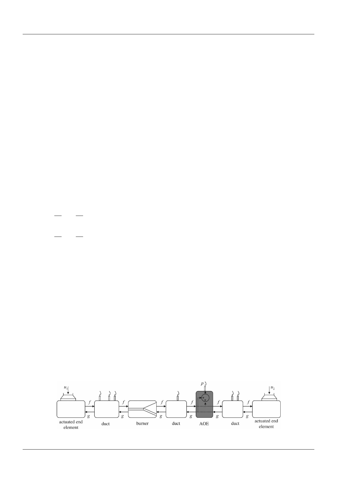
acoustic test rig. Figure 1 shows a schematic overview

of the experimental facility.

The model for the test rig is split into subsystems,

whose scattering matrices were determined exper-

imentally (burner, up-, and downstream end) and

analytically (ducts). Interconnection of the subsys-

tems yields a model for the test rig, which can be used

to predict its acoustic field.

The up- and downstream ends are equipped with

circumferentially mounted loudspeakers, which allow

for acoustic excitation of the rig. With these loud-

speakers, it is possible to adjust the linearly indepen-

dent test states that are necessary to experimentally

obtain a system’s scattering matrix. For the determi-

nation of the acoustic field, the test rig’s duct sections

are instrumented with 1/4 condenser microphones.

There are three microphones upstream of the burner

element and four downstream, thus allowing for the

application of the MMM.

4.2 Setup of the simulation model

4.2.1 Loudspeaker elements

The speaker elements’ transfer functions were deter-

mined experimentally. The elements have two inputs

and one output. In the case of the upstream element,

the g-wave and the loudspeaker voltage u1are the

inputs while the f-wave represents the output. In the

frequency domain this can be written as

f=Rg +Gu1(6)

where Ris the reflection coefficient and Gthe transfer

function of the loudspeaker’s controlling input volt-

age to the outgoing f-wave. Equation (6) implies the

assumption that the contribution of the reflection

coefficient and the loudspeaker transfer function can

be linearly superimposed. Results shown in section 4.3

confirm the validity of this assumption.

Similar to the approach described previously, two

excitation states have to be generated. This is achieved

using loudspeaker excitation at each side separately.

Downstream excitation (index A) yields

fA=RgA(7)

from equation (6) as u1is zero. This allows for direct

calculation of the reflection coefficient R. Excitation

Fig. 1 Schematic overview of the acoustic test rig splitted up into its subsystems

Modelling and analysis of complex thermoacoustic systems 661

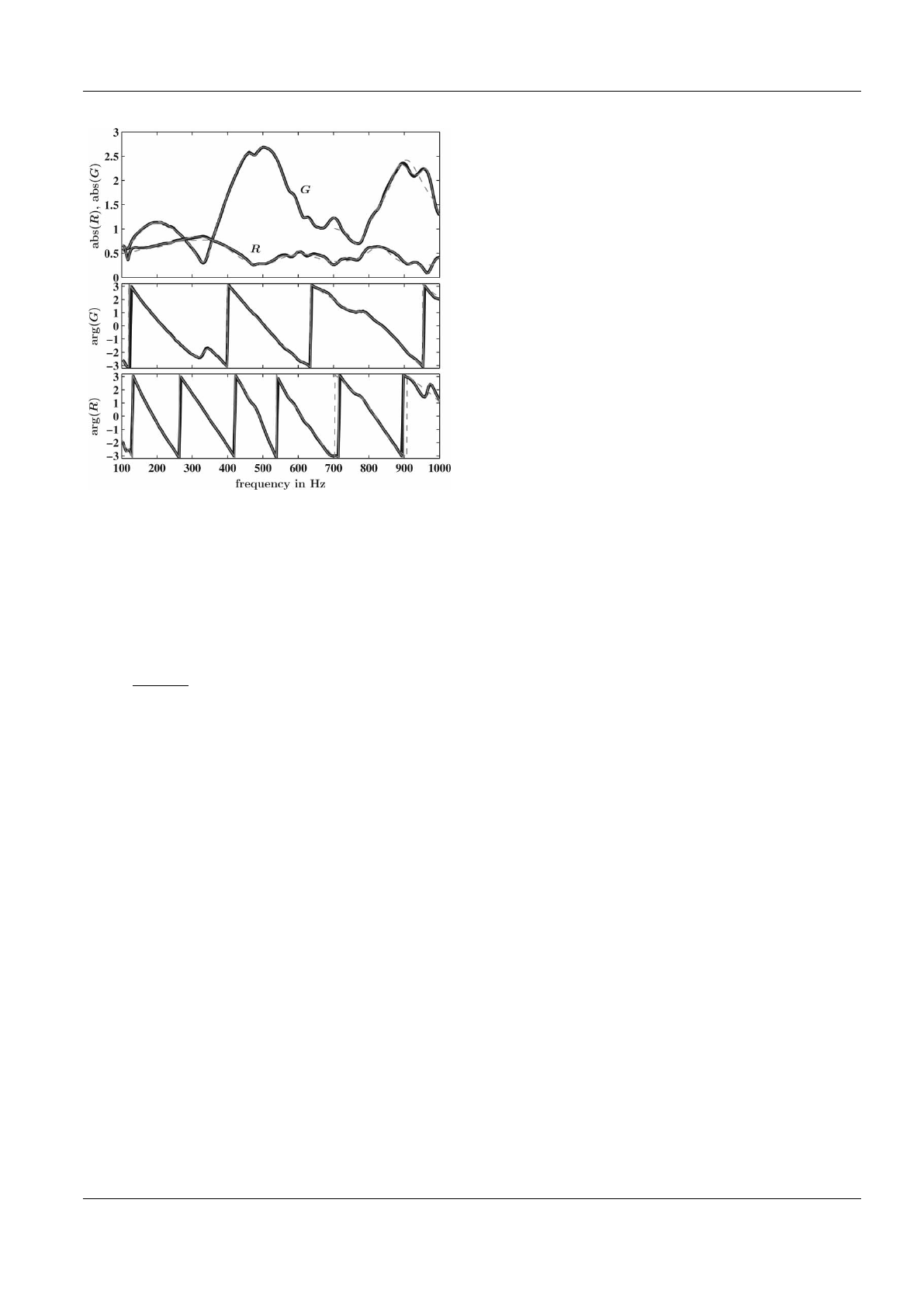
Fig. 2 Loudspeaker transfer function (G) and reflection

coefficient (R) for measured values (black), model

with 30 states (grey), and model with 15 states

(grey dashed). Top: absolute value, middle: phase

of G, bottom: phase of R

with the upstream loudspeaker (index B) and solving

for Ggives

G=fB−RgB

(8)

where Ris calculated from equation (7).

With complex values for Rand Gcalculated at

discrete frequencies, frequency domain system iden-

tification algorithms [26,27] were used to obtain

state-space models. As stated before, the frequency-

dependent transfer functions are approximated by

partial fraction expansions. The number of poles used

for this expansion determines the number of states

of the state-space system. Figure 2 depicts gain and

phase of Rand G. Results for measured data as

well as for models identified with 30 states and 15

states are shown.

As can be seen in Fig. 2, measured and computed

curves for gain and phase of the reflection coefficient R

modelled with 30 states match almost perfectly. In the

frequency regime above 700 Hz, the model obtained

with 15 states shows minor deviations. In the case of

the loudspeaker’s transfer function G, excellent results

are obtained with 30 states. With 15 states, the results

are fair except for some frequency bands, in which G

has several local extremal values. Regarding the phase,

both models agree well with the measured values. The

larger slope of R, i.e. the larger time-delay, is due to

the position of the loudspeaker. The incident wave

travels to the upstream element’s end and back to

the reference plane, whereas the emitted wave of the

loudspeaker has to travel a much shorter distance.

Up to this point, only two SISO state-space systems

exist. These have to be concatenated to a double input

single output state-space system, which completely

describes the upstream end

x=AR0

0AGx+BR0

0BGg

u1

f=[CRCG]x+[DRDG]g

u1(9)

Indices Rand Gdenote the matrices of the reflec-

tion coefficient’s and the loudspeaker’s state-space

systems, respectively.

4.2.2 Artificial output element

The grey highlighted element in Fig. 1, is not part of

the real system but only an artificial component of the

model system. Through this, it is possible to access

the signal of any microphone by placing the artificial

output element (AOE) at the position of the desired

microphone. The element is modelled in state-space

as a static gain without additional dynamics

⎡

⎣

⎤

⎦=⎡

⎣

⎤

⎦fu

gd(10)

Besides the Dmatrix, all other matrices of the state-

space system (A,B, and C) are empty. The output

element has a physical length of zero. The up- and

downstream travelling waves are neither delayed nor

changed in amplitude and therefore, the output ele-

ment does not influence the acoustic behaviour of the

total system.

4.2.3 Interconnected complete system

The outputs of each subsystem have to be con-

nected with the inputs of its adjacent subsystems.

Linking together the subsystems’ state-space repre-

sentations results in one single state-space model for

the complete system. The interconnection is exem-

plarily shown for two adjacent subsystems of the

acoustic test rig.

The transfer behaviour of a subsystem defines the

relation betweenincidentandoutgoingwaves.Bycon-

necting the two subsystems‘duct’ and‘burner’ (Fig. 3),

one system is obtained with the Riemann invariants f1

and g3as inputs and g1and f3as outputs. Thus, the

two systems of equations describing the individual

subsystems are now combined to one, representing

the transfer behaviour of the connected system. This

combination is a matrix operation referred to as the

Loading more pages...