Modeling of orientational polarization within the framework of extended micropolar theory [original]

Continuum Mech. Thermodyn. (2021) 33:1263–1279

https://doi.org/10.1007/s00161-021-00972-x

ORIGINAL ARTICLE

Elena N. Vilchevskaya ·Wolfgang H. Müller

Modeling of orientational polarization within the framework

of extended micropolar theory

Received: 2 October 2020 / Accepted: 7 January 2021 / Published online: 28 January 2021

Abstract In this paper the process of polarization of transversally polarizable matter is investigated based on

concepts from micropolar theory. The process is modeled as a structural change of a dielectric material. On

the microscale it is assumed that it consists of rigid dipoles subjected to an external electric field, which leads

to a certain degree of ordering. The ordering is limited, because it is counteracted by thermal motion, which

favors stochastic orientation of the dipoles. An extended balance equation for the microinertia tensor is used

to model these effects. This balance contains a production term. The constitutive equations for this term are

split into two parts, one , which accounts for the orienting effect of the applied external electric field, and

another one, which is used to represent chaotic thermal motion. Two relaxation times are used to characterize

the impact of each term on the temporal development. In addition homogenization techniques are applied in

order to determine the final state of polarization. The traditional homogenization is based on calculating the

average effective length of polarized dipoles. In a non-traditional approach the inertia tensor of the rigid rods

is homogenized. Both methods lead to similar results. The final states of polarization are then compared with

the transient simulation. By doing so it becomes possible to link the relaxation times to the finally observed

state of order, which in terms of the finally obtained polarization is a measurable quantity.

1 Polarization in dielectrics modeled by extended micropolar theory

Extended micropolar theory is capable of modeling structural changes in materials. The orientational polar-

ization of a dielectric can be considered as a structural change and is, therefore, a suitable candidate for this

kind of modeling. The paper is organized as follows. In this section we will present the basic relations of

micropolar theory, first, in general terms, and then, in particular, focus on a discussion of its extension. The

next section will, first, mostly for the benefit of the mechanics community, provide a short recapitulation of the

phenomenon of electric polarization, in particular orientational polarization. Second the equations of extended

micropolar theory will be specialized to the requirement of its modeling. In particular we shall specify the

required production term based on physical grounds. Moreover, Sect. 2presents homogenization procedures

that allow to capture the final state of polarization. These results can then be linked to the modeling of the

Communicated by Marcus Aßmus, Victor A. Eremeyev and Andreas Öchsner.

E. N. Vilchevskaya

Institute for Problems in Mechanical Engineering of the Russian Academy of Sciences, Bol’shoy pr. 61, V.O., 199178 St.

Petersburg, Russia

W. H. Müller (B)

Institute of Mechanics, Chair of Continuum Mechanics and Constitutive Theory, Technische Universität Berlin, Sekr. MS. 2,

Einsteinufer 5, 10587 Berlin, Germany

E-mail: [email protected]

1264 E. N. Vilchevskaya, W. H. Müller

temporal evolution of polarization obtainable within the framework of extended micropolar theory. The paper

will end with a summary and an outlook into further applications based on the presented results.

1.1 Introductory remarks: Benefits of the concept of the microinertia tensor

Traditionally the microinertia tensor of a continuum particle, J, plays an important role only in context with

its rotational degrees of freedom. In combination with the angular velocity vector, ω, it characterizes the

spin of the continuum element. The details are outlined in Eringen’s theory of micropolar media, see for

example [11]. There it is shown that the microinertia tensor obeys a kinematic constraint in form of a rate

equation, which expresses the possibility of material continuum particles to undergo rigid body rotations.

This feature is captured by means of three rotating rigid directors. Within the framework of this theory the

shape of the microinertia tensor does not change; rather, it can only rotate rigidly. Eringen calls such materials

micropolar media. However, as we shall demonstrate in this paper, describing the particle spin is not the

only use of the microinertia tensor. If generalized, the concept of a changing microinertia can be beneficial

for describing processes in certain materials, for example, electromagnetic ones, such as the development of

electricpolarization,whichmayalreadyoccurundertheabsenceofanangularvelocity.Someotherapplications

of micropolar theory can be found, for example, in [3,4].

In fact a radical change of the concept of the microinertia tensor has been presented recently in [14]. There

the microinertia tensor is treated as a completely independent field variable for solid and fluid matter alike.

In this formulation closed as well as open systems are allowed. This means that in- and outflux of matter in a

Representative Volume Element (RVE) can be taken into account and the concept of a material particle is not

imperative. Moreover, a structural change due to external forces becomes possible. The microinertia tensor

becomes a fully independent field variable with its own balance requiring additional constitutive quantities.

More specifically, in contrast with the balance of mass, the balance for the micro-inertia tensor is not conserved.

It contains a production term, χ, which could be specified by following the rules of constitutive theory or be

motivated by physics and intuition, such that fundamental principles are not violated.

In the following subsections it will be demonstrated that this extended theory allows for the modeling of

processes accompanied by a considerable structural change characterized by a changing microinertia within

a representative volume element, such as the development of orientational polarization in matter under the

action of an external electric field, E. In this context the multi-disciplinary aspect of the present formulation

should be stressed. Potentially it can be used fruitfully to synthesize new innovative materials [34], which

combinemechanicalandelectricalbehavior.Forexample,theuseofpiezoelectricpatchescanprovidereduction

in vibrations or energy harvesting (see, e.g., [2,12]). Moreover, for a recent thermodynamically consistent

treatment of electro-mechanical problems see [1].

1.2 The balances of micropolar media

The motion and state of micropolar media in spatial description are described by the following coupled system

of differential equations:

•balance of mass,

δρ

δt=−ρ∇·v,(1.1)

•balance of momentum,

δv

δt=∇·σ+ρf,(1.2)

•balance of spin,

ρJ·δω

δt=−ρω×J·ω+∇·μ+σ×+ρm,(1.3)

•balance of internal energy,

δu

δt=σ:∇v+I×ω+μ:∇ω−∇·q+ρr,(1.4)

Modeling of orientational polarization 1265

where ρis the field of mass density, vand ωare the linear and angular velocity fields, σis the non-symmetric

Cauchy stress tensor, fis the specific body force, Jis the specific micro-inertia tensor, μis the non-symmetric

couple stress tensor, (ab)×=a×bis the Gibbsian cross, mare specific body couples, uis the specific

internal energy, qis the heat flux, and ris the specific heat supply. By the colon we denote the outer double

scalar product between tensors of second rank, A:B=AijBij. Moreover,

δ(·)

δt=d(·)

dt+(v−w)·∇(·)(1.5)

is the substantial derivative of a field quantity, d(·)

/dtthe total derivative, and wthe mapping velocity of the

observational point (see [13]).

It was already indicated that traditional micropolar theory assumes that each material point or “particle”

of a micropolar continuum is phenomenologically equivalent to a rigid body. It can rotate but the state of the

rotational inertia in the principal axes system does not change. In other words the micro-inertia tensor will not

change its form nor shape, see, for example, [9], [32], [19], [11]. Even if a so-called micromorphic medium

is considered, which in principle allows an intrinsic change of micro-inertia (following [8], [11], [10]), many

publications use only the following additional equation for the conservation of inertia (e.g., see [23], [5]),

which is an identity of rigid body kinematics:

δJ

δt=ω×J−J×ω.(1.6)

Noteagainthatthetermson the right-hand sidecharacterizethechangeof the inertia tensor,whichisexclusively

due to rigid body rotation.

An extension to this approach was suggested in [7], where it was proposed that the microinertia of polar

particles may change as the continuum deforms. This idea was then further elaborated in [14], where it was

clearly stated that the tensor of microinertia should be treated as an independent field. Within that approach a

fixedand openelementary volume Vwastreatedas a micropolar continuum (macro-) region,as it iscustomarily

done in spatial description. Then its microinertia tensor J(in units of m2) as a property on the continuum

scale is obtained by homogenization as follows. Within the elementary volume Vthere are i=1, ..., N

microparticles of mass miand inertia tensor ˆ

Ji(in units of kgm2) such that:

m=1



i=1

mi,J=1



i=1ˆ

Ji,(1.7)

where mis the average mass within V. If the linear and angular velocities of the particles are denoted by vi

and ωi, then the specific linear and angular momenta are given by:

v=1



i=1

mivi,J·ω=1



i=1ˆ

Ji·ωi⇒ω=N



i=1ˆ

Ji−1



i=1ˆ

Ji·ωi.(1.8)

The specific linear momentum is nothing else but the translational velocity on the continuum scale. Equation

(1.8)1simplifies considerably if all the microparticles have the same mass:

v=1



i=1

vi.(1.9)

This will be the case for the dielectric medium considered in this paper. Moreover, we will also assume that

the inertia tensors of the microparticles are the “same.” This means that the three principal values of the inertia

tensor are the same for each particle, ˆ

i=ˆ

Jj, but its eigensystem vectors e∗

i,j,j=1,2,3 are not, because

the microparticles are randomly oriented. Thus, in such a case we can only say that

Ji=ˆ

J1e∗

i,1e∗

i,1+ˆ

J2e∗

i,2e∗

i,2+ˆ

J3e∗

i,3e∗

i,3⇒J= ˆ

m.(1.10)

1266 E. N. Vilchevskaya, W. H. Müller

Only for a spherical inertia tensor, or if all microparticles are aligned in the same manner, the last relation

would turn into an equality. This also means that in all other cases of “equal” inertia tensors we must conclude

from the last relation in (1.8)that

ω= 1



i=1

ωi.(1.11)

Because of the movement of the medium, the elementary volume contains different microparticles as time

passes, and the microinertia tensor assigned to the volume will change due to the incoming or outgoing flux of

inertia. However, internal structural transformations are also possible. These can be due to (a) the combination

or fragmentation of the particles during mechanical crushing, to (b) chemical reactions, or to (c) changes of the

anisotropy of the material, for example by applying external electromagnetic fields. Such effects are explained

in greater detail in [22], [21], [20], or [33]. In a nutshell, on the continuum scale all of this can be taken into

account by adding a source or production term, χ, to the right-hand side of Eq. (1.6), which now reads:

δJ

δt=ω×J−J×ω+χ.(1.12)

On the continuum level this source term must be considered as a new constitutive quantity for which an

additional constitutive equation has to be formulated. The form of the constitutive equation depends on the

problem under consideration and can be a function of many physical quantities. A suitable form for the

modeling of orientational polarization in polarizable matter under the influence of an external electric field

will be discussed in the next section.

Finally it should be emphasized once more that the field of microinertia, i.e., the rotational inertia of the

continuum influences the development of the angular velocity ω. The temporal development is dictated by the

spin balance (1.3), and this is usually the only purpose of J. In this paper it is different: Because of the extended

balance (1.12)Jcan also be used to characterize structural changes of the micropolar medium, without the

presence of an angular velocity. We proceed to explain this in more detail in the next section.

2 Polarization modeling

2.1 Introductory remarks on polarization

For didactical reasons we recapitulate a few facts from electrical engineering in this section. In this field one

distinguishes between electrically conducting and non-conducting or insulating materials. On a microscopic

scale the former possess freely movable electric charges, for example the electron gas in metals. In case of the

latter charges cannot move around freely. Positive and negative charges must stay together. They are bound

within a molecule or other basic atomic units, for example within a crystal lattice. Materials in which an electric

current cannot flow are also known as dielectrics. In the absence of external electric fields they are electrically

neutral. However, one of their basic properties is the ability to polarize if an external electric field Eis applied.

This leads to the creation of surface charges, which on the continuum scale are described by the polarization

vector P. Indeed, ∂VP·ndAallows to compute that charge, provided the field Pis known.

The question arises how the polarization can be measured, at least in principle, since a direct measurement

of charges, in particular surface charges, is difficult. A simple school experiment can be used. Consider a

plate capacitor, which is first charged by a battery, so that the plates of surface Aat a distance dare loaded

with the electric charges ±Q. The battery is then detached and replaced by a voltmeter. If there is vacuum in

between the plates, the voltmeter will show a voltage Uvac, say. If we now place a dielectric body in between

this voltage decreases down to Upol <Uvac. The stronger the decrease, the more surface charges are created,

and the stronger the polarization Pwill be. In order to quantify the effect in terms of a material constant, let

us assume for simplicity that the dielectric material between the plates is isotropic and the polarization vector

can be described by a linear constitutive equation of the type:

P=ε0χE,(2.1)

where ε0=8.854 ×10−12 As

Vm is the electric field constant and χ>0 is the dielectric susceptibility, which

in this simple case is a material-dependent, dimensionless constant. In fact, application of the static Maxwell

Modeling of orientational polarization 1267

Fig. 1 Polarization types adapted after [16]

equations to the case of the plate capacitor described above yields:

Upol =Qd

ε0(1+χ)A.(2.2)

The combination εr=1+χis also known as relative permittivity, which is also dimensionless. It is equal to

one for the case of vacuum. Then Eq. (2.2) allows to determine εror χif the the two voltages before and after

filling the vacuum are measured:

χ=Uvac

Upol −1.(2.3)

Note that if the dielectric is anisotropic and if the electric field is not too high, the dielectric suscep-

tibility constant can simply be replaced by a constant second rank dielectric susceptibility tensor, χ.For

large electric fields the dielectric susceptibility is a nonlinear function of the electric field, χ(E),which

is sometimes expressed in a power series. Moreover, analogously to viscoelasticity, which makes use of a

frequency-dependent complex shear modulus during harmonic loading, it becomes necessary to introduce

a frequency-dependent and complex valued dielectric susceptibility when harmonically alternating electric

fields are applied.

It should be emphasized that we made these remarks just to illustrate the measurement principle. In practice

(frequency dependent) susceptibilities and relative permittivities are measured dynamically, for example, by

using microwave waveguide systems, see [35].

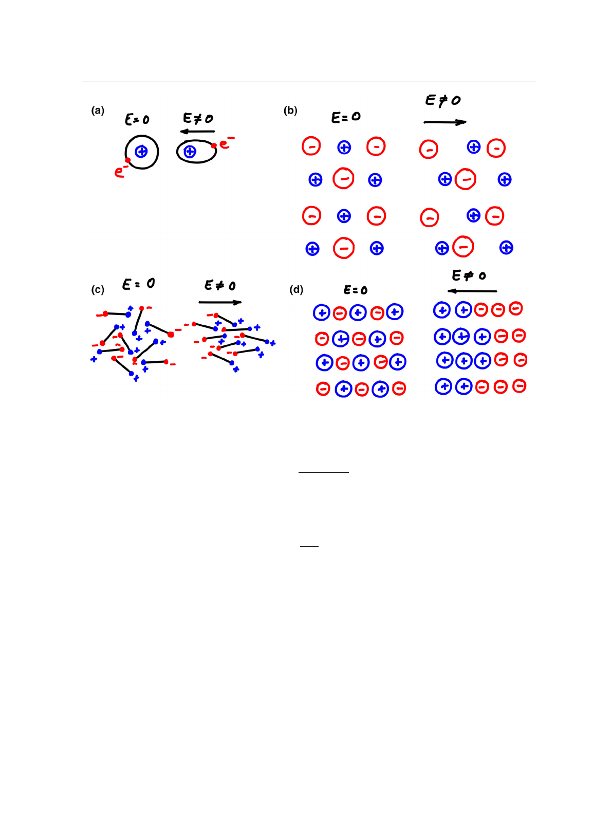
Figure 1presents cartoons of the various polarization mechanisms encountered in materials on the

microscale.

Inset (a) refers to electronic polarization. Due to the electric field the positive charge of the atomic nucleus

and the negative charge of the surrounding electron cloud are shifted with respect to each other so that an

atomic dipole results. If the field is removed, the electron cloud and the nucleus move reversibly into their

old position. The atom is electrically neutral and no longer a dipole. It is a very weak effect in (more or less

Loading more pages...