
Technische Universit¨at Berlin
Institut f¨ur Mathematik
Regularization and Numerical Simulation
of Dynamical Systems Modeled with
Modelica
Randolf Altmeyer∗ ‡ and Andreas Steinbrecher† ‡
Preprint 2013/29
Preprint-Reihe des Instituts f¨ur Mathematik
Technische Universit¨at Berlin
Report 2013/29 September 2013

Quasi-linear differential-algebraic equations (DAEs) are essential tools for
modeling dynamical processes, e.g. for mechanical systems, electrical circuits
or chemical reactions. These models are in general of higher index and contain
so called hidden constraints which lead to instabilities and order reductions
during numerical integration of the model equations.
In this article we consider dynamical systems modeled with quasi-linear
DAEs of higher index using Modelica. We investigate a regularization of
model equations in the Modelica framework in view of an efficient and robust
numerical simulation.
We will present an approach for numerical integration of quasi-linear DAEs
which is based on overdetermined DAEs obtained from dynamical models
modeled with Modelica.
AMS(MOS) subject classification: 34A09, 65K05, 65L80
Keywords: dynamical systems, differential-algebraic equations, regular-
ization, numerical integration, Modelica, QUALIDAES, MO2FOR
Authors address:
Randolf Altmeyer
Institut f¨ur Mathematik
Humboldt Universit¨at zu Berlin
10099 Berlin, Germany
Andreas Steinbrecher
Institut f¨ur Mathematik, MA 4–5,
Technische Universit¨at Berlin
Str. des 17. Juni 136
10623 Berlin, Germany

Regularization and Numerical Simulation of
Dynamical Systems Modeled with Modelica
Randolf Altmeyer∗‡ and Andreas Steinbrecher†‡
September 30, 2013
Abstract
Quasi-linear differential-algebraic equations (DAEs) are essential tools
for modeling dynamical processes, e.g. for mechanical systems, electrical
circuits or chemical reactions. These models are in general of higher index
and contain so called hidden constraints which lead to instabilities and
order reductions during numerical integration of the model equations.
In this article we consider dynamical systems modeled with quasi-linear
DAEs of higher index using Modelica. We investigate a regularization of
model equations in the Modelica framework in view of an efficient and
robust numerical simulation.
We will present an approach for numerical integration of quasi-linear
DAEs which is based on overdetermined DAEs obtained from dynami-
cal models modeled with Modelica.
Keywords: dynamical systems, differential-algebraic equations, reg-
ularization, numerical integration, Modelica, QUALIDAES, MO2FOR
AMS(MOS) subject classification: 34A09, 65K05, 65L80
1 Introduction
The modeling of dynamical processes, like electrical circuits, multibody systems,
thermal systems or flow problems often leads to model equations of differential
equations with algebraic constraints, so called differential-algebraic equations
(DAEs). For modeling such dynamical processes the modeling language Mod-
elica [4] is a common and useful tool. Modelica is an object-oriented language
for complex systems containing several subsystems, e.g., mechanical, electrical,
or hydraulic subcomponents. There exists a large variety of modeling and sim-
ulation tools, e.g., OpenModelica1, Dymola2, MapleSim3, SimulationX4.
∗Institut f¨ur Mathematik, Humboldt Universit¨at zu Berlin, 10099 Berlin, Germany;
†Institut f¨ur Mathematik, TU Berlin, Straße des 17. Juni 136, 10623 Berlin, Germany;
‡The author’s work was supported by the ERC Advanced Grant ”Modeling, Simulation
and Control of Multi-Physics Systems” MODSIMCONMP
1https://www.openmodelica.org
2http://www.dymola.com
3http://www.maplesoft.com/products/maplesim/
4http://www.simulationx.com
1

To investigate the dynamical behaviour the model equations have to be inte-
grated. The solution of such DAEs is restricted to satisfy algebraic constraints
contained in the DAE. But in general not all constraints are stated in an explicit
way in the DAE. In general there exist so called hidden constraints leading to
a higher index. Therefore, the numerical treatment of DAEs is nontrivial in
general and more complicated than for ordinary differential equations (ODEs),
see [2, 10, 12, 13]. Among the effects arising from hidden constraints are insta-
bilities, convergence problems or inconsistencies, for instance.
A way out of the dilemma of hidden constraints in model equations is to remodel
or regularize the dynamical system, see for instance [6, 9, 12, 13, 19, 20].
The dynamical system is often modeled as initial value problem for quasi-linear
DAEs
E(x, t) ˙x=k(x, t),(1)
on the domain I= [t0, tf] with initial values x(t0) = x0∈Rn,where E∈ C(Rn×
I,Rn,n) is called the leading matrix of the quasi-linear DAE and k∈ C(Rn×I,Rn)
its right-hand side. Furthermore, x:I→Rnrepresents the unknown variables.
The equations are assumed to be uniquely solvable for consistent initial values
and nonredundant. In this article we restrict our considerations to quasi-linear
DAEs (1) where we assume that the rank of the leading matrix Eis constant
for all (x, t)∈Rn×Iand, furthermore, the rank of the partial derivatives of the
(hidden) constraints with respect to xis constant for all (x, t)∈Rn×I. Note
that in general these assumptions are not necessary and can be relaxed, see [18].
As a special case of the quasi-linear DAE (1), we will investigate semi-implicit
DAEs of the form
E1(x, t) ˙x=k1(x, t),(2a)
0 = k2(x, t) (2b)
with E1∈ C(Rn×I,Rm1,n), k1∈ C(Rn×I,Rm1) and k2∈ C(Rn×I,Rm2). We
assume m1+m2≥n.
In the following, for a differentiable time dependent function xwe denote the
total derivative with respect to tby ˙x(t)=dx(t)/dt. For a differentiable function
fdepending on xthe (partial) derivative of f(x) with respect to xis denoted by
f,x(x) = ∂
∂x f(x). The same notation is used for differentiable vector functions.
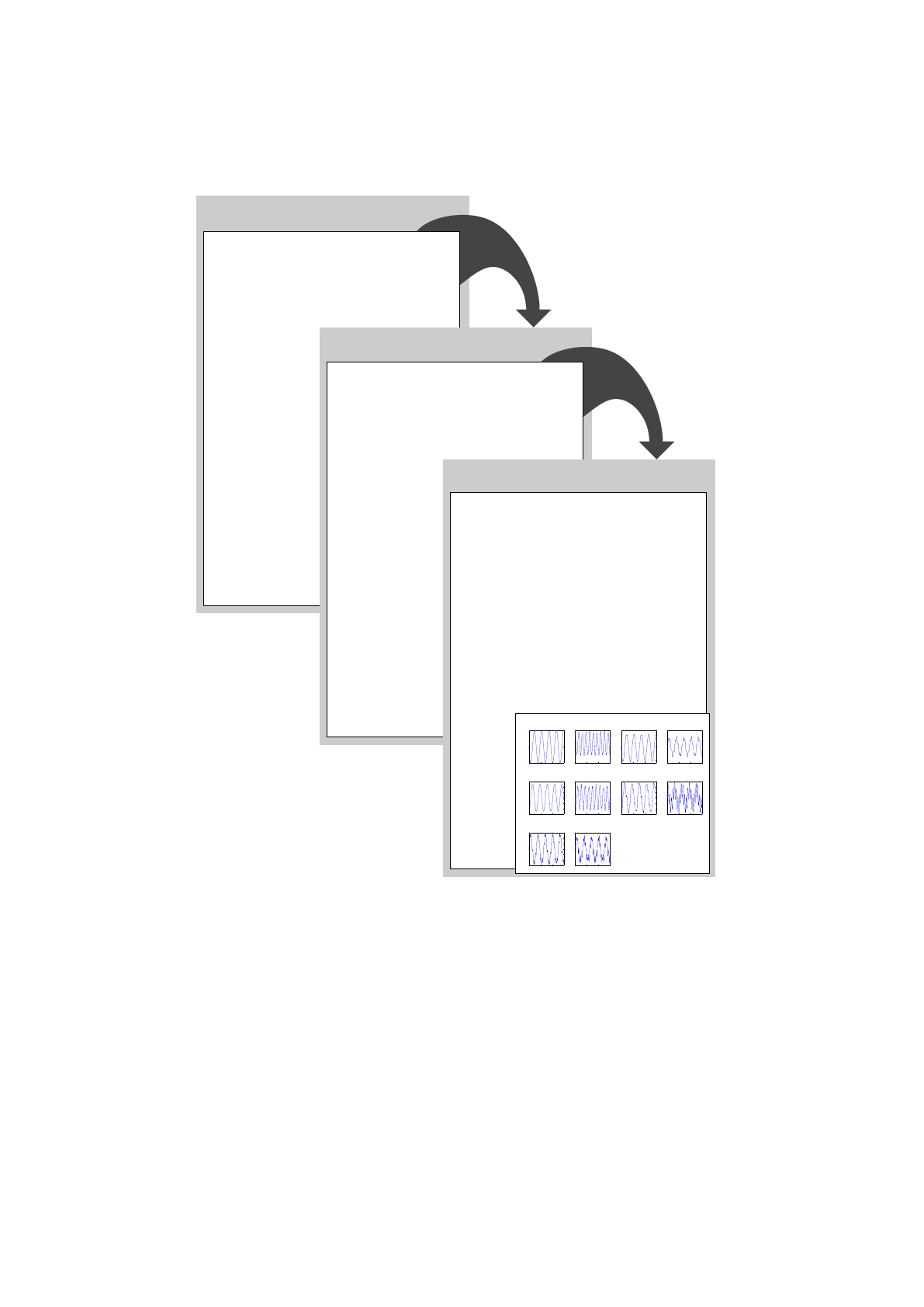
In this article we will discuss an approach for regularization and numerical inte-
gration of dynamical systems modeled with Modelica as illustrated in Figure 1.
The first step consists of regularizing the model equations, via overdetermined
formulations including all hidden constraints, see Section 2, while the second
step performs the subsequent robust and efficient numerical integration using
the Runge-Kutta method RADAU IIa of order 5, see Section 3. The combined
approach of regularization and subsequent numerical integration is implemented
in the software package MO2FOR/QUALIDAES which we present in Section 4. The
applicability of MO2FOR/QUALIDAES for the numerical treatment of model equa-
tions provided in Modelica language is demonstrated at the example of a simple
pendulum and of a car axis in Section 5.
2
class CarAxis
parameter Real eps=0.01,M=10,L=1,L0=0.5,r=0.1,w=10;
Real xl(start=0),yl(start=0.5),
xr(start=1),yr(start=0.5),
V1(start=-0.5),V2(start=0),V3(start=-0.5),V4(start=0),
lam1(start=0),lam2(start=0),
V1P(start=0),V2P(start=0),V3P(start=0),V4P(start=0),
yb(start=0),ybP(start=1),ybPP(start=0),
xb(start=1),xbP(start=0),xbPP(start=-1),
Ll(start=0.5),Lr(start=0.5);
equation
//abreviations//
yb = r *sin(w*time);
ybP = r*w *cos(w*time);
ybPP=-r*w*w*sin(w*time);
xb = (L*L-yb*yb)^0.5;
xbP =-yb*ybP/(L*L-yb*yb)^0.5;
xbPP=-yb*yb*ybP*ybP/(L*L-yb*yb)^1.5
-(ybP*ybP+yb*ybPP)/(L*L-yb*yb)^0.5;
Ll = (xl^2+yl^2)^0.5;
Lr = ((xr-xb)^2+(yr-yb)^2)^0.5;
V1P =(L0-Ll)*xl/Ll +lam1*xb+2*lam2*(xl-xr);
V2P =(L0-Ll)*yl/Ll +lam1*yb+2*lam2*(yl-yr)-M*eps*eps/2;
V3P =(L0-Lr)*(xr-xb)/Lr -2*lam2*(xl-xr);
V4P =(L0-Lr)*(yr-yb)/Lr -2*lam2*(yl-yr)-M*eps*eps/2;
//kinematic equations of motion//
der(xl) = V1;
der(yl) = V2;
der(xr) = V3;
der(yr) = V4;
//dynamic equations of motion//
eps*eps*M/2*der(V1) =V1P;
eps*eps*M/2*der(V2) =V2P;
eps*eps*M/2*der(V3) =V3P;
eps*eps*M/2*der(V4) =V4P;
//constraints on position level//
0 = xb*xl+yb*yl;
0 = (xl-xr)^2+(yl-yr)^2-L*L;
//constraints on velocity level//
0 = xbP*xl+xb*V1+ybP*yl+yb*V2;
0 = 2*(xl-xr)*(V1-V3)+2*(yl-yr)*(V2-V4);
//constraints on acceleration level//
0 = xbPP*xl+2*xbP*V1+xb*V1P/(eps*eps*M/2)
+ybPP*yl+2*ybP*V2+yb*V2P/(eps*eps*M/2);
0 = 2*(V1-V3)*(V1-V3)
+2*(xl-xr)*(V1P-V3P)/(eps*eps*M/2)
+2*(V2-V4)*(V2-V4)
+2*(yl-yr)*(V2P-V4P)/(eps*eps*M/2);
end CarAxis;
Model Equations
in Modelica Source Code Regularization
and
Translation
with
MO2FOR
C CarAxis
C Solver: Qualidaes
DOUBLE PRECISION qT,qTSTART,qTEND,qH,qH0,qCPT0,qCPT1,qPERT
PARAMETER (eps=0.01D0,M=10.0D0,L=1.0D0,L0=0.5D0,r=0.1D0,w=10.0D0)
...
CALL QUALIDAES(
# qMD,qMC,qN,qNIVCOND,
# qX,qT,qTEND,qH,qRTOL,qATOL,qITOL,qIOPT,qROPT,
...
END
C
SUBROUTINE RHS(qMD,qMC,qN,qT,qX,qF,qG,qIOPT,qROPT,qIPAR,qRPAR,qIDI
#D)
C
INTEGER qMD,qMC,qN,qIOPT(*),qIPAR(*),qIDID
DOUBLE PRECISION qT,qX(qN),qF(qMD),qG(qMC),qROPT(*),qRPAR(*)
...
xl = qX(1)!
yl = qX(2)!
xr = qX(3)!
C
qF(1) = V1
qF(2) = V2
...
qF(7) = V3P
qF(8) = V4P
qG(1) = -yb+r*Dsin(w*qT)
qG(2) = -ybP+r*w*Dcos(w*qT)
...
qG(17) = xbPP*xl+2.0D0*xbP*V1+xb*V1P/((eps*eps*M/(2.0D0)))+ybPP*yl
#+2.0D0*ybP*V2+yb*V2P/((eps*eps*M/(2.0D0)))
qG(18) = 2.0D0*(V1-V3)*(V1-V3)+2.0D0*(xl-xr)*(V1P-V3P)/((eps*eps*M
#/(2.0D0)))+2.0D0*(V2-V4)*(V2-V4)+2.0D0*(yl-yr)*(V2P-V4P)/((eps*eps
#*M/(2.0D0)))
END
C
SUBROUTINE MATRIX(qMD,qN,qT,qX,qMA,qIOPT,qROPT,qIPAR,qRPAR,qIDID)
C
INTEGER qMD,qN,qI,qJ,qIOPT(*),qIPAR(*),qIDID
DOUBLE PRECISION qT,qX(qN),qMA(qMD,qN),qROPT(*),qRPAR(*)
...
qMA(1,1) = 1.0D0
qMA(2,2) = 1.0D0
...
qMA(7,7) = eps*eps*M/(2.0D0)
qMA(8,8) = eps*eps*M/(2.0D0)
C
END
Overdetermined Formulation
in Fortran Source Code Numerical
Integration
with
QUALIDAES
simvar={’T’;’xl’;’yl’;’xr’;’yr’;’V1’;’V2’;’V3’;’V4’;’lam1’;’lam2’;’V1P’;...
simres( 1,:)=[ 0.0000000000000000D+00, 0.0000000000000000D+00, 0.500...
simres( 2,:)=[ 0.3000000000000000D-02,-0.1499768249498017D-02, 0.499...
simres( 3,:)=[ 0.6000000000000000D-02,-0.2998146715500600D-02, 0.499...
simres( 4,:)=[ 0.9000000000000001D-02,-0.4493747897578716D-02, 0.499...
simres( 5,:)=[ 0.1200000000000000D-01,-0.5985190001019940D-02, 0.499...
simres( 6,:)=[ 0.1500000000000000D-01,-0.7471097948602796D-02, 0.499...
simres( 7,:)=[ 0.1800000000000000D-01,-0.8950107967364899D-02, 0.499...
simres( 8,:)=[ 0.2100000000000000D-01,-0.1042086632660879D-01, 0.499...
simres( 9,:)=[ 0.2400000000000000D-01,-0.1188203574468467D-01, 0.499...
simres( 10,:)=[ 0.2700000000000000D-01,-0.1333229140304438D-01, 0.499...
simres( 11,:)=[ 0.3000000000000000D-01,-0.1477032717129503D-01, 0.499...
simres( 12,:)=[ 0.3300000000000000D-01,-0.1619485463241374D-01, 0.499...
simres( 13,:)=[ 0.3600000000000000D-01,-0.1760459968823099D-01, 0.499...
simres( 14,:)=[ 0.3900000000000000D-01,-0.1899831324399283D-01, 0.499...
simres( 15,:)=[ 0.4200000000000000D-01,-0.2037476046201573D-01, 0.499...
simres( 16,:)=[ 0.4500000000000000D-01,-0.2173272542109633D-01, 0.499...
simres( 17,:)=[ 0.4800000000000000D-01,-0.2307101880316631D-01, 0.499...
simres( 18,:)=[ 0.5100000000000000D-01,-0.2438846541859802D-01, 0.498...
...
simres( 987,:)=[ 0.2958000000000000D+01, 0.4820124685925711D-01, 0.497...
simres( 988,:)=[ 0.2961000000000000D+01, 0.4857183713944243D-01, 0.497...
simres( 989,:)=[ 0.2964000000000000D+01, 0.4889872768180634D-01, 0.497...
simres( 990,:)=[ 0.2967000000000000D+01, 0.4918162068660767D-01, 0.497...
simres( 991,:)=[ 0.2970000000000000D+01, 0.4942025026404851D-01, 0.497...
simres( 992,:)=[ 0.2973000000000000D+01, 0.4961440494976911D-01, 0.496...
simres( 993,:)=[ 0.2976000000000000D+01, 0.4976391375329137D-01, 0.496...
simres( 994,:)=[ 0.2979000000000000D+01, 0.4986864032525427D-01, 0.496...
simres( 995,:)=[ 0.2982000000000000D+01, 0.4992850424407702D-01, 0.496...
simres( 996,:)=[ 0.2985000000000000D+01, 0.4994345257951636D-01, 0.496...
simres( 997,:)=[ 0.2988000000000000D+01, 0.4991347696390285D-01, 0.496...
simres( 998,:)=[ 0.2991000000000000D+01, 0.4983861375609260D-01, 0.496...
simres( 999,:)=[ 0.2994000000000000D+01, 0.4971892681580792D-01, 0.496...
simres( 1000,:)=[ 0.2997000000000000D+01, 0.4955453100876348D-01, 0.496...
simres( 1001,:)=[ 0.3000000000000000D+01, 0.4934557505765604D-01, 0.496...
IDID= 0;
T= 3.0000;
NACCPT = 412;
NRHS = 3518;
NPDEC = 384;
NERJCT = 43;
NJAC = 384;
NEDEC = 433;
NCRJCT = 0;
NMAT = 3516;
NBSUB = 1044;
CPUTIME= 0.076;
NSEL = 1;
Numerical Results
0 1 2 3
−0.05
0
0.05
Position xl
0 1 2 3
0.496
0.497
0.498
0.499
0.5
Position yl
0 1 2 3
0.95
1
1.05
Position xr
0 1 2 3
0.3
0.4
0.5
0.6
Position yl
0 1 2 3
−0.4
−0.2
0
0.2
0.4
0.6
Velocity for xl
0 1 2 3
−0.04
−0.02
0
0.02
0.04
Velocity for yl
0 1 2 3
−0.4
−0.2
0
0.2
0.4
0.6
Velocity for xr
0 1 2 3
−2
−1
0
1
2
Velocity for yl
0 1 2 3
−6
−4
−2
0
2
4
6
x 10−3
Lagr. Mult. λ1
0 1 2 3
−2
−1
0
1
2
x 10−3
Lagr. Mult. λ2
Figure 1: Scheme MO2FOR -QUALIDAES
2 Regularization using Overdetermined Formu-
lations
In general, the solution of higher index DAEs is not only restricted by explicit
constraints, as for instance in (2b), but also by so called hidden constraints
which are not explicitly stated as equations, see [18]. These constraints im-
pose additional consistency conditions on the initial values and on the solution,
thereby causing problems for direct numerical integration of DAEs of higher
index, see [1, 2, 6, 8, 10, 11, 12, 15, 16].
3
Loading more pages...